BOCS AdaptiveBOCS Adaptive Strategy - Automated Volatility Breakout System
WHAT THIS STRATEGY DOES:
This is an automated trading strategy that detects consolidation patterns through volatility analysis and executes trades when price breaks out of these channels. Take-profit and stop-loss levels are calculated dynamically using Average True Range (ATR) to adapt to current market volatility. The strategy closes positions partially at the first profit target and exits the remainder at the second target or stop loss.
TECHNICAL METHODOLOGY:
Price Normalization Process:
The strategy begins by normalizing price to create a consistent measurement scale. It calculates the highest high and lowest low over a user-defined lookback period (default 100 bars). The current close price is then normalized using the formula: (close - lowest_low) / (highest_high - lowest_low). This produces values between 0 and 1, allowing volatility analysis to work consistently across different instruments and price levels.
Volatility Detection:
A 14-period standard deviation is applied to the normalized price series. Standard deviation measures how much prices deviate from their average - higher values indicate volatility expansion, lower values indicate consolidation. The strategy uses ta.highestbars() and ta.lowestbars() functions to track when volatility reaches peaks and troughs over the detection length period (default 14 bars).
Channel Formation Logic:
When volatility crosses from a high level to a low level, this signals the beginning of a consolidation phase. The strategy records this moment using ta.crossover(upper, lower) and begins tracking the highest and lowest prices during the consolidation. These become the channel boundaries. The duration between the crossover and current bar must exceed 10 bars minimum to avoid false channels from brief volatility spikes. Channels are drawn using box objects with the recorded high/low boundaries.
Breakout Signal Generation:
Two detection modes are available:
Strong Closes Mode (default): Breakout occurs when the candle body midpoint math.avg(close, open) exceeds the channel boundary. This filters out wick-only breaks.
Any Touch Mode: Breakout occurs when the close price exceeds the boundary.
When price closes above the upper channel boundary, a bullish breakout signal generates. When price closes below the lower boundary, a bearish breakout signal generates. The channel is then removed from the chart.
ATR-Based Risk Management:
The strategy uses request.security() to fetch ATR values from a specified timeframe, which can differ from the chart timeframe. For example, on a 5-minute chart, you can use 1-minute ATR for more responsive calculations. The ATR is calculated using ta.atr(length) with a user-defined period (default 14).
Exit levels are calculated at the moment of breakout:
Long Entry Price = Upper channel boundary
Long TP1 = Entry + (ATR × TP1 Multiplier)
Long TP2 = Entry + (ATR × TP2 Multiplier)
Long SL = Entry - (ATR × SL Multiplier)
For short trades, the calculation inverts:
Short Entry Price = Lower channel boundary
Short TP1 = Entry - (ATR × TP1 Multiplier)
Short TP2 = Entry - (ATR × TP2 Multiplier)
Short SL = Entry + (ATR × SL Multiplier)
Trade Execution Logic:
When a breakout occurs, the strategy checks if trading hours filter is satisfied (if enabled) and if position size equals zero (no existing position). If volume confirmation is enabled, it also verifies that current volume exceeds 1.2 times the 20-period simple moving average.
If all conditions are met:
strategy.entry() opens a position using the user-defined number of contracts
strategy.exit() immediately places a stop loss order
The code monitors price against TP1 and TP2 levels on each bar
When price reaches TP1, strategy.close() closes the specified number of contracts (e.g., if you enter with 3 contracts and set TP1 close to 1, it closes 1 contract). When price reaches TP2, it closes all remaining contracts. If stop loss is hit first, the entire position exits via the strategy.exit() order.
Volume Analysis System:
The strategy uses ta.requestUpAndDownVolume(timeframe) to fetch up volume, down volume, and volume delta from a specified timeframe. Three display modes are available:
Volume Mode: Shows total volume as bars scaled relative to the 20-period average
Comparison Mode: Shows up volume and down volume as separate bars above/below the channel midline
Delta Mode: Shows net volume delta (up volume - down volume) as bars, positive values above midline, negative below
The volume confirmation logic compares breakout bar volume to the 20-period SMA. If volume ÷ average > 1.2, the breakout is classified as "confirmed." When volume confirmation is enabled in settings, only confirmed breakouts generate trades.
INPUT PARAMETERS:
Strategy Settings:
Number of Contracts: Fixed quantity to trade per signal (1-1000)
Require Volume Confirmation: Toggle to only trade signals with volume >120% of average
TP1 Close Contracts: Exact number of contracts to close at first target (1-1000)
Use Trading Hours Filter: Toggle to restrict trading to specified session
Trading Hours: Session input in HHMM-HHMM format (e.g., "0930-1600")
Main Settings:
Normalization Length: Lookback bars for high/low calculation (1-500, default 100)
Box Detection Length: Period for volatility peak/trough detection (1-100, default 14)
Strong Closes Only: Toggle between body midpoint vs close price for breakout detection
Nested Channels: Allow multiple overlapping channels vs single channel at a time
ATR TP/SL Settings:
ATR Timeframe: Source timeframe for ATR calculation (1, 5, 15, 60, etc.)
ATR Length: Smoothing period for ATR (1-100, default 14)
Take Profit 1 Multiplier: Distance from entry as multiple of ATR (0.1-10.0, default 2.0)
Take Profit 2 Multiplier: Distance from entry as multiple of ATR (0.1-10.0, default 3.0)
Stop Loss Multiplier: Distance from entry as multiple of ATR (0.1-10.0, default 1.0)
Enable Take Profit 2: Toggle second profit target on/off
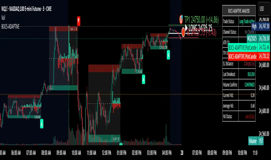
VISUAL INDICATORS:
Channel boxes with semi-transparent fill showing consolidation zones
Green/red colored zones at channel boundaries indicating breakout areas
Volume bars displayed within channels using selected mode
TP/SL lines with labels showing both price level and distance in points
Entry signals marked with up/down triangles at breakout price
Strategy status table showing position, contracts, P&L, ATR values, and volume confirmation status
HOW TO USE:
For 2-Minute Scalping:
Set ATR Timeframe to "1" (1-minute), ATR Length to 12, TP1 Multiplier to 2.0, TP2 Multiplier to 3.0, SL Multiplier to 1.5. Enable volume confirmation and strong closes only. Use trading hours filter to avoid low-volume periods.
For 5-15 Minute Day Trading:
Set ATR Timeframe to match chart or use 5-minute, ATR Length to 14, TP1 Multiplier to 2.0, TP2 Multiplier to 3.5, SL Multiplier to 1.2. Volume confirmation recommended but optional.
For Hourly+ Swing Trading:
Set ATR Timeframe to 15-30 minute, ATR Length to 14-21, TP1 Multiplier to 2.5, TP2 Multiplier to 4.0, SL Multiplier to 1.5. Volume confirmation optional, nested channels can be enabled for multiple setups.
BACKTEST CONSIDERATIONS:
Strategy performs best during trending or volatility expansion phases
Consolidation-heavy or choppy markets produce more false signals
Shorter timeframes require wider stop loss multipliers due to noise
Commission and slippage significantly impact performance on sub-5-minute charts
Volume confirmation generally improves win rate but reduces trade frequency
ATR multipliers should be optimized for specific instrument characteristics
COMPATIBLE MARKETS:
Works on any instrument with price and volume data including forex pairs, stock indices, individual stocks, cryptocurrency, commodities, and futures contracts. Requires TradingView data feed that includes volume for volume confirmation features to function.
KNOWN LIMITATIONS:
Stop losses execute via strategy.exit() and may not fill at exact levels during gaps or extreme volatility
request.security() on lower timeframes requires higher-tier TradingView subscription
False breakouts inherent to breakout strategies cannot be completely eliminated
Performance varies significantly based on market regime (trending vs ranging)
Partial closing logic requires sufficient position size relative to TP1 close contracts setting
RISK DISCLOSURE:
Trading involves substantial risk of loss. Past performance of this or any strategy does not guarantee future results. This strategy is provided for educational purposes and automated backtesting. Thoroughly test on historical data and paper trade before risking real capital. Market conditions change and strategies that worked historically may fail in the future. Use appropriate position sizing and never risk more than you can afford to lose. Consider consulting a licensed financial advisor before making trading decisions.
ACKNOWLEDGMENT & CREDITS:
This strategy is built upon the channel detection methodology created by AlgoAlpha in the "Smart Money Breakout Channels" indicator. Full credit and appreciation to AlgoAlpha for pioneering the normalized volatility approach to identifying consolidation patterns and sharing this innovative technique with the TradingView community. The enhancements added to the original concept include automated trade execution, multi-timeframe ATR-based risk management, partial position closing by contract count, volume confirmation filtering, and real-time position monitoring.
Cari dalam skrip untuk "stop loss"
Optimized ADX DI CCI Strategy### Key Features:
- Combines ADX, DI+/-, CCI, and RSI for signal generation.
- Supports customizable timeframes for indicators.
- Offers multiple exit conditions (Moving Average cross, ADX change, performance-based stop-loss).
- Tracks and displays trade statistics (e.g., win rate, capital growth, profit factor).
- Visualizes trades with labels and optional background coloring.
- Allows countertrading (opening an opposite trade after closing one).
1. **Indicator Calculation**:
- **ADX and DI+/-**: Calculated using the `ta.dmi` function with user-defined lengths for DI and ADX smoothing.
- **CCI**: Computed using the `ta.cci` function with a configurable source (default: `hlc3`) and length.
- **RSI (optional)**: Calculated using the `ta.rsi` function to filter overbought/oversold conditions.
- **Moving Averages**: Used for CCI signal smoothing and trade exits, with support for SMA, EMA, SMMA (RMA), WMA, and VWMA.
2. **Signal Generation**:
- **Buy Signal**: Triggered when DI+ > DI- (or DI+ crosses over DI-), CCI > MA (or CCI crosses over MA), and optional ADX/RSI filters are satisfied.
- **Sell Signal**: Triggered when DI+ < DI- (or DI- crosses over DI+), CCI < MA (or CCI crosses under MA), and optional ADX/RSI filters are satisfied.
3. **Trade Execution**:
- **Entry**: Long or short trades are opened using `strategy.entry` when signals are detected, provided trading is allowed (`allow_long`/`allow_short`) and equity is positive.
- **Exit**: Trades can be closed based on:
- Opposite signal (if no other exit conditions are used).
- MA cross (price crossing below/above the exit MA for long/short trades).
- ADX percentage change exceeding a threshold.
- Performance-based stop-loss (trade loss exceeding a percentage).
- **Countertrading**: If enabled, closing a trade triggers an opposite trade (e.g., closing a long opens a short).
4. **Visualization**:
- Labels are plotted at trade entries/exits (e.g., "BUY," "SELL," arrows).
- Optional background coloring highlights open trades (green for long, red for short).
- A statistics table displays real-time metrics (e.g., capital, win rates).
5. **Trade Tracking**:
- Tracks the number of long/short trades, wins, and overall performance.
- Monitors equity to prevent trading if it falls to zero.
### 2.3 Key Components
- **Indicator Calculations**: Uses `request.security` to fetch indicator data for the specified timeframe.
- **MA Function**: A custom `ma_func` handles different MA types for CCI and exit conditions.
- **Signal Logic**: Combines crossover/under checks with recent bar windows for flexibility.
- **Exit Conditions**: Multiple configurable exit strategies for risk management.
- **Statistics Table**: Updates dynamically with trade and capital metrics.
## 3. Configuration Options
The script provides extensive customization through input parameters, grouped for clarity in the TradingView settings panel. Below is a detailed breakdown of each setting and its impact.
### 3.1 Strategy Settings (Global)
- **Initial Capital**: Default `10000`. Sets the starting capital for backtesting.
- **Effect**: Determines the base equity for calculating position sizes and performance metrics.
- **Default Quantity Type**: `strategy.percent_of_equity` (50% of equity).
- **Effect**: Controls the size of each trade as a percentage of available equity.
- **Pyramiding**: Default `2`. Allows up to 2 simultaneous trades in the same direction.
- **Effect**: Enables multiple entries if conditions are met, increasing exposure.
- **Commission**: 0.2% per trade.
- **Effect**: Simulates trading fees, reducing net profit in backtesting.
- **Margin**: 100% for long and short trades.
- **Effect**: Assumes no leverage; adjust for margin trading simulations.
- **Calc on Every Tick**: `true`.
- **Effect**: Ensures real-time signal updates for precise execution.
### 3.2 Indicator Settings
- **Indicator Timeframe** (`indicator_timeframe`):
- **Options**: `""` (chart timeframe), `1`, `5`, `15`, `30`, `60`, `240`, `D`, `W`.
- **Default**: `""` (uses chart timeframe).
- **Effect**: Determines the timeframe for ADX, DI, CCI, and RSI calculations. A higher timeframe reduces noise but may delay signals.
### 3.3 ADX & DI Settings
- **DI Length** (`adx_di_len`):
- **Default**: `30`.
- **Range**: Minimum `1`.
- **Effect**: Sets the period for calculating DI+ and DI-. Longer periods smooth trends but reduce sensitivity.
- **ADX Smoothing Length** (`adx_smooth_len`):
- **Default**: `14`.
- **Range**: Minimum `1`.
- **Effect**: Smooths the ADX calculation. Longer periods produce smoother ADX values.
- **Use ADX Filter** (`use_adx_filter`):
- **Default**: `false`.
- **Effect**: If `true`, requires ADX to exceed the threshold for signals to be valid, filtering out weak trends.
- **ADX Threshold** (`adx_threshold`):
- **Default**: `25`.
- **Range**: Minimum `0`.
- **Effect**: Sets the minimum ADX value for valid signals when the filter is enabled. Higher values restrict trades to stronger trends.
### 3.4 CCI Settings
- **CCI Length** (`cci_length`):
- **Default**: `20`.
- **Range**: Minimum `1`.
- **Effect**: Sets the period for CCI calculation. Longer periods reduce noise but may lag.
- **CCI Source** (`cci_src`):
- **Default**: `hlc3` (average of high, low, close).
- **Effect**: Defines the price data for CCI. `hlc3` is standard, but users can choose other sources (e.g., `close`).
- **CCI MA Type** (`ma_type`):
- **Options**: `SMA`, `EMA`, `SMMA (RMA)`, `WMA`, `VWMA`.
- **Default**: `SMA`.
- **Effect**: Determines the moving average type for CCI signal smoothing. EMA is more responsive; VWMA weights by volume.
- **CCI MA Length** (`ma_length`):
- **Default**: `14`.
- **Range**: Minimum `1`.
- **Effect**: Sets the period for the CCI MA. Longer periods smooth the MA but may delay signals.
### 3.5 RSI Filter Settings
- **Use RSI Filter** (`use_rsi_filter`):
- **Default**: `false`.
- **Effect**: If `true`, applies RSI-based overbought/oversold filters to signals.
- **RSI Length** (`rsi_length`):
- **Default**: `14`.
- **Range**: Minimum `1`.
- **Effect**: Sets the period for RSI calculation. Longer periods reduce sensitivity.
- **RSI Lower Limit** (`rsi_lower_limit`):
- **Default**: `30`.
- **Range**: `0` to `100`.
- **Effect**: Defines the oversold threshold for buy signals. Lower values allow trades in more extreme conditions.
- **RSI Upper Limit** (`rsi_upper_limit`):
- **Default**: `70`.
- **Range**: `0` to `100`.
- **Effect**: Defines the overbought threshold for sell signals. Higher values allow trades in more extreme conditions.
### 3.6 Signal Settings
- **Cross Window** (`cross_window`):
- **Default**: `0`.
- **Range**: `0` to `5` bars.
- **Effect**: Specifies the lookback period for detecting DI+/- or CCI crosses. `0` requires crosses on the current bar; higher values allow recent crosses, increasing signal frequency.
- **Allow Long Trades** (`allow_long`):
- **Default**: `true`.
- **Effect**: Enables/disables new long trades. If `false`, only closing existing longs is allowed.
- **Allow Short Trades** (`allow_short`):
- **Default**: `true`.
- **Effect**: Enables/disables new short trades. If `false`, only closing existing shorts is allowed.
- **Require DI+/DI- Cross for Buy** (`buy_di_cross`):
- **Default**: `true`.
- **Effect**: If `true`, requires a DI+ crossover DI- for buy signals; if `false`, DI+ > DI- is sufficient.
- **Require CCI Cross for Buy** (`buy_cci_cross`):
- **Default**: `true`.
- **Effect**: If `true`, requires a CCI crossover MA for buy signals; if `false`, CCI > MA is sufficient.
- **Require DI+/DI- Cross for Sell** (`sell_di_cross`):
- **Default**: `true`.
- **Effect**: If `true`, requires a DI- crossover DI+ for sell signals; if `false`, DI+ < DI- is sufficient.
- **Require CCI Cross for Sell** (`sell_cci_cross`):
- **Default**: `true`.
- **Effect**: If `true`, requires a CCI crossunder MA for sell signals; if `false`, CCI < MA is sufficient.
- **Countertrade** (`countertrade`):
- **Default**: `true`.
- **Effect**: If `true`, closing a trade triggers an opposite trade (e.g., close long, open short) if allowed.
- **Color Background for Open Trades** (`color_background`):
- **Default**: `true`.
- **Effect**: If `true`, colors the chart background green for long trades and red for short trades.
### 3.7 Exit Settings
- **Use MA Cross for Exit** (`use_ma_exit`):
- **Default**: `true`.
- **Effect**: If `true`, closes trades when the price crosses the exit MA (below for long, above for short).
- **MA Length for Exit** (`ma_exit_length`):
- **Default**: `20`.
- **Range**: Minimum `1`.
- **Effect**: Sets the period for the exit MA. Longer periods delay exits.
- **MA Type for Exit** (`ma_exit_type`):
- **Options**: `SMA`, `EMA`, `SMMA (RMA)`, `WMA`, `VWMA`.
- **Default**: `SMA`.
- **Effect**: Determines the MA type for exit signals. EMA is more responsive; VWMA weights by volume.
- **Use ADX Change Stop-Loss** (`use_adx_stop`):
- **Default**: `false`.
- **Effect**: If `true`, closes trades when the ADX changes by a specified percentage.
- **ADX % Change for Stop-Loss** (`adx_change_percent`):
- **Default**: `5.0`.
- **Range**: Minimum `0.0`, step `0.1`.
- **Effect**: Specifies the percentage change in ADX (vs. previous bar) that triggers a stop-loss. Higher values reduce premature exits.
- **Use Performance Stop-Loss** (`use_perf_stop`):
- **Default**: `false`.
- **Effect**: If `true`, closes trades when the loss exceeds a percentage threshold.
- **Performance Stop-Loss (%)** (`perf_stop_percent`):
- **Default**: `-10.0`.
- **Range**: `-100.0` to `0.0`, step `0.1`.
- **Effect**: Specifies the loss percentage that triggers a stop-loss. More negative values allow larger losses before exiting.
## 4. Visual and Statistical Output
- **Labels**: Displayed at trade entries/exits with arrows (↑ for buy, ↓ for sell) and text ("BUY," "SELL"). A "No Equity" label appears if equity is zero.
- **Background Coloring**: Optionally colors the chart background (green for long, red for short) to indicate open trades.
- **Statistics Table**: Displayed at the top center of the chart, updated on timeframe changes or trade events. Includes:
- **Capital Metrics**: Initial capital, current capital, capital growth (%).
- **Trade Metrics**: Total trades, long/short trades, win rate, long/short win rates, profit factor.
- **Open Trade Status**: Indicates if a long, short, or no trade is open.
## 5. Alerts
- **Buy Signal Alert**: Triggered when `buy_signal` is true ("Cross Buy Signal").
- **Sell Signal Alert**: Triggered when `sell_signal` is true ("Cross Sell Signal").
- **Usage**: Users can set up TradingView alerts to receive notifications for trade signals.

VoVix DEVMA🌌 VoVix DEVMA: A Deep Dive into Second-Order Volatility Dynamics
Welcome to VoVix+, a sophisticated trading framework that transcends traditional price analysis. This is not merely another indicator; it is a complete system designed to dissect and interpret the very fabric of market volatility. VoVix+ operates on the principle that the most powerful signals are not found in price alone, but in the behavior of volatility itself. It analyzes the rate of change, the momentum, and the structure of market volatility to identify periods of expansion and contraction, providing a unique edge in anticipating major market moves.
This document will serve as your comprehensive guide, breaking down every mathematical component, every user input, and every visual element to empower you with a profound understanding of how to harness its capabilities.
🔬 THEORETICAL FOUNDATION: THE MATHEMATICS OF MARKET DYNAMICS
VoVix+ is built upon a multi-layered mathematical engine designed to measure what we call "second-order volatility." While standard indicators analyze price, and first-order volatility indicators (like ATR) analyze the range of price, VoVix+ analyzes the dynamics of the volatility itself. This provides insight into the market's underlying state of stability or chaos.
1. The VoVix Score: Measuring Volatility Thrust
The core of the system begins with the VoVix Score. This is a normalized measure of volatility acceleration or deceleration.
Mathematical Formula:
VoVix Score = (ATR(fast) - ATR(slow)) / (StDev(ATR(fast)) + ε)
Where:
ATR(fast) is the Average True Range over a short period, representing current, immediate volatility.
ATR(slow) is the Average True Range over a longer period, representing the baseline or established volatility.
StDev(ATR(fast)) is the Standard Deviation of the fast ATR, which measures the "noisiness" or consistency of recent volatility.
ε (epsilon) is a very small number to prevent division by zero.
Market Implementation:
Positive Score (Expansion): When the fast ATR is significantly higher than the slow ATR, it indicates a rapid increase in volatility. The market is "stretching" or expanding.
Negative Score (Contraction): When the fast ATR falls below the slow ATR, it indicates a decrease in volatility. The market is "coiling" or contracting.
Normalization: By dividing by the standard deviation, we normalize the score. This turns it into a standardized measure, allowing us to compare volatility thrust across different market conditions and timeframes. A score of 2.0 in a quiet market means the same, relatively, as a score of 2.0 in a volatile market.
2. Deviation Analysis (DEV): Gauging Volatility's Own Volatility
The script then takes the analysis a step further. It calculates the standard deviation of the VoVix Score itself.
Mathematical Formula:
DEV = StDev(VoVix Score, lookback_period)
Market Implementation:
This DEV value represents the magnitude of chaos or stability in the market's volatility dynamics. A high DEV value means the volatility thrust is erratic and unpredictable. A low DEV value suggests the change in volatility is smooth and directional.
3. The DEVMA Crossover: Identifying Regime Shifts
This is the primary signal generator. We take two moving averages of the DEV value.
Mathematical Formula:
fastDEVMA = SMA(DEV, fast_period)
slowDEVMA = SMA(DEV, slow_period)
The Core Signal:
The strategy triggers on the crossover and crossunder of these two DEVMA lines. This is a profound concept: we are not looking at a moving average of price or even of volatility, but a moving average of the standard deviation of the normalized rate of change of volatility.
Bullish Crossover (fastDEVMA > slowDEVMA): This signals that the short-term measure of volatility's chaos is increasing relative to the long-term measure. This often precedes a significant market expansion and is interpreted as a bullish volatility regime.
Bearish Crossunder (fastDEVMA < slowDEVMA): This signals that the short-term measure of volatility's chaos is decreasing. The market is settling down or contracting, often leading to trending moves or range consolidation.
⚙️ INPUTS MENU: CONFIGURING YOUR ANALYSIS ENGINE
Every input has been meticulously designed to give you full control over the strategy's behavior. Understanding these settings is key to adapting VoVix+ to your specific instrument, timeframe, and trading style.
🌀 VoVix DEVMA Configuration
🧬 Deviation Lookback: This sets the lookback period for calculating the DEV value. It defines the window for measuring the stability of the VoVix Score. A shorter value makes the system highly reactive to recent changes in volatility's character, ideal for scalping. A longer value provides a smoother, more stable reading, better for identifying major, long-term regime shifts.
⚡ Fast VoVix Length: This is the lookback period for the fastDEVMA. It represents the short-term trend of volatility's chaos. A smaller number will result in a faster, more sensitive signal line that reacts quickly to market shifts.
🐌 Slow VoVix Length: This is the lookback period for the slowDEVMA. It represents the long-term, baseline trend of volatility's chaos. A larger number creates a more stable, slower-moving anchor against which the fast line is compared.
How to Optimize: The relationship between the Fast and Slow lengths is crucial. A wider gap (e.g., 20 and 60) will result in fewer, but potentially more significant, signals. A narrower gap (e.g., 25 and 40) will generate more frequent signals, suitable for more active trading styles.
🧠 Adaptive Intelligence
🧠 Enable Adaptive Features: When enabled, this activates the strategy's performance tracking module. The script will analyze the outcome of its last 50 trades to calculate a dynamic win rate.
⏰ Adaptive Time-Based Exit: If Enable Adaptive Features is on, this allows the strategy to adjust its Maximum Bars in Trade setting based on performance. It learns from the average duration of winning trades. If winning trades tend to be short, it may shorten the time exit to lock in profits. If winners tend to run, it will extend the time exit, allowing trades more room to develop. This helps prevent the strategy from cutting winning trades short or holding losing trades for too long.
⚡ Intelligent Execution
📊 Trade Quantity: A straightforward input that defines the number of contracts or shares for each trade. This is a fixed value for consistent position sizing.
🛡️ Smart Stop Loss: Enables the dynamic stop-loss mechanism.
🎯 Stop Loss ATR Multiplier: Determines the distance of the stop loss from the entry price, calculated as a multiple of the current 14-period ATR. A higher multiplier gives the trade more room to breathe but increases risk per trade. A lower multiplier creates a tighter stop, reducing risk but increasing the chance of being stopped out by normal market noise.
💰 Take Profit ATR Multiplier: Sets the take profit target, also as a multiple of the ATR. A common practice is to set this higher than the Stop Loss multiplier (e.g., a 2:1 or 3:1 reward-to-risk ratio).
🏃 Use Trailing Stop: This is a powerful feature for trend-following. When enabled, instead of a fixed stop loss, the stop will trail behind the price as the trade moves into profit, helping to lock in gains while letting winners run.
🎯 Trail Points & 📏 Trail Offset ATR Multipliers: These control the trailing stop's behavior. Trail Points defines how much profit is needed before the trail activates. Trail Offset defines how far the stop will trail behind the current price. Both are based on ATR, making them fully adaptive to market volatility.
⏰ Maximum Bars in Trade: This is a time-based stop. It forces an exit if a trade has been open for a specified number of bars, preventing positions from being held indefinitely in stagnant markets.
⏰ Session Management
These inputs allow you to confine the strategy's trading activity to specific market hours, which is crucial for day trading instruments that have defined high-volume sessions (e.g., stock market open).
🎨 Visual Effects & Dashboard
These toggles give you complete control over the on-chart visuals and the dashboard. You can disable any element to declutter your chart or focus only on the information that matters most to you.
📊 THE DASHBOARD: YOUR AT-A-GLANCE COMMAND CENTER
The dashboard centralizes all critical information into one compact, easy-to-read panel. It provides a real-time summary of the market state and strategy performance.
🎯 VOVIX ANALYSIS
Fast & Slow: Displays the current numerical values of the fastDEVMA and slowDEVMA. The color indicates their direction: green for rising, red for falling. This lets you see the underlying momentum of each line.
Regime: This is your most important environmental cue. It tells you the market's current state based on the DEVMA relationship. 🚀 EXPANSION (Green) signifies a bullish volatility regime where explosive moves are more likely. ⚛️ CONTRACTION (Purple) signifies a bearish volatility regime, where the market may be consolidating or entering a smoother trend.
Quality: Measures the strength of the last signal based on the magnitude of the DEVMA difference. An ELITE or STRONG signal indicates a high-conviction setup where the crossover had significant force.
PERFORMANCE
Win Rate & Trades: Displays the historical win rate of the strategy from the backtest, along with the total number of closed trades. This provides immediate feedback on the strategy's historical effectiveness on the current chart.
EXECUTION
Trade Qty: Shows your configured position size per trade.
Session: Indicates whether trading is currently OPEN (allowed) or CLOSED based on your session management settings.
POSITION
Position & PnL: Displays your current position (LONG, SHORT, or FLAT) and the real-time Profit or Loss of the open trade.
🧠 ADAPTIVE STATUS
Stop/Profit Mult: In this simplified version, these are placeholders. The primary adaptive feature currently modifies the time-based exit, which is reflected in how long trades are held on the chart.
🎨 THE VISUAL UNIVERSE: DECIPHERING MARKET GEOMETRY
The visuals are not mere decorations; they are geometric representations of the underlying mathematical concepts, designed to give you an intuitive feel for the market's state.
The Core Lines:
FastDEVMA (Green/Maroon Line): The primary signal line. Green when rising, indicating an increase in short-term volatility chaos. Maroon when falling.
SlowDEVMA (Aqua/Orange Line): The baseline. Aqua when rising, indicating a long-term increase in volatility chaos. Orange when falling.
🌊 Morphism Flow (Flowing Lines with Circles):
What it represents: This visualizes the momentum and strength of the fastDEVMA. The width and intensity of the "beam" are proportional to the signal strength.
Interpretation: A thick, steep, and vibrant flow indicates powerful, committed momentum in the current volatility regime. The floating '●' particles represent kinetic energy; more particles suggest stronger underlying force.
📐 Homotopy Paths (Layered Transparent Boxes):
What it represents: These layered boxes are centered between the two DEVMA lines. Their height is determined by the DEV value.
Interpretation: This visualizes the overall "volatility of volatility." Wider boxes indicate a chaotic, unpredictable market. Narrower boxes suggest a more stable, predictable environment.
🧠 Consciousness Field (The Grid):
What it represents: This grid provides a historical lookback at the DEV range.
Interpretation: It maps the recent "consciousness" or character of the market's volatility. A consistently wide grid suggests a prolonged period of chaos, while a narrowing grid can signal a transition to a more stable state.
📏 Functorial Levels (Projected Horizontal Lines):
What it represents: These lines extend from the current fastDEVMA and slowDEVMA values into the future.
Interpretation: Think of these as dynamic support and resistance levels for the volatility structure itself. A crossover becomes more significant if it breaks cleanly through a prior established level.
🌊 Flow Boxes (Spaced Out Boxes):
What it represents: These are compact visual footprints of the current regime, colored green for Expansion and red for Contraction.
Interpretation: They provide a quick, at-a-glance confirmation of the dominant volatility flow, reinforcing the background color.
Background Color:
This provides an immediate, unmistakable indication of the current volatility regime. Light Green for Expansion and Light Aqua/Blue for Contraction, allowing you to assess the market environment in a split second.
📊 BACKTESTING PERFORMANCE REVIEW & ANALYSIS
The following is a factual, transparent review of a backtest conducted using the strategy's default settings on a specific instrument and timeframe. This information is presented for educational purposes to demonstrate how the strategy's mechanics performed over a historical period. It is crucial to understand that these results are historical, apply only to the specific conditions of this test, and are not a guarantee or promise of future performance. Market conditions are dynamic and constantly change.
Test Parameters & Conditions
To ensure the backtest reflects a degree of real-world conditions, the following parameters were used. The goal is to provide a transparent baseline, not an over-optimized or unrealistic scenario.
Instrument: CME E-mini Nasdaq 100 Futures (NQ1!)
Timeframe: 5-Minute Chart
Backtesting Range: March 24, 2024, to July 09, 2024
Initial Capital: $100,000
Commission: $0.62 per contract (A realistic cost for futures trading).
Slippage: 3 ticks per trade (A conservative setting to account for potential price discrepancies between order placement and execution).
Trade Size: 1 contract per trade.
Performance Overview (Historical Data)
The test period generated 465 total trades , providing a statistically significant sample size for analysis, which is well above the recommended minimum of 100 trades for a strategy evaluation.
Profit Factor: The historical Profit Factor was 2.663 . This metric represents the gross profit divided by the gross loss. In this test, it indicates that for every dollar lost, $2.663 was gained.
Percent Profitable: Across all 465 trades, the strategy had a historical win rate of 84.09% . While a high figure, this is a historical artifact of this specific data set and settings, and should not be the sole basis for future expectations.
Risk & Trade Characteristics
Beyond the headline numbers, the following metrics provide deeper insight into the strategy's historical behavior.
Sortino Ratio (Downside Risk): The Sortino Ratio was 6.828 . Unlike the Sharpe Ratio, this metric only measures the volatility of negative returns. A higher value, such as this one, suggests that during this test period, the strategy was highly efficient at managing downside volatility and large losing trades relative to the profits it generated.
Average Trade Duration: A critical characteristic to understand is the strategy's holding period. With an average of only 2 bars per trade , this configuration operates as a very short-term, or scalping-style, system. Winning trades averaged 2 bars, while losing trades averaged 4 bars. This indicates the strategy's logic is designed to capture quick, high-probability moves and exit rapidly, either at a profit target or a stop loss.
Conclusion and Final Disclaimer
This backtest demonstrates one specific application of the VoVix+ framework. It highlights the strategy's behavior as a short-term system that, in this historical test on NQ1!, exhibited a high win rate and effective management of downside risk. Users are strongly encouraged to conduct their own backtests on different instruments, timeframes, and date ranges to understand how the strategy adapts to varying market structures. Past performance is not indicative of future results, and all trading involves significant risk.
🔧 THE DEVELOPMENT PHILOSOPHY: FROM VOLATILITY TO CLARITY
The journey to create VoVix+ began with a simple question: "What drives major market moves?" The answer is often not a change in price direction, but a fundamental shift in market volatility. Standard indicators are reactive to price. We wanted to create a system that was predictive of market state. VoVix+ was designed to go one level deeper—to analyze the behavior, character, and momentum of volatility itself.
The challenge was twofold. First, to create a robust mathematical model to quantify these abstract concepts. This led to the multi-layered analysis of ATR differentials and standard deviations. Second, to make this complex data intuitive and actionable. This drove the creation of the "Visual Universe," where abstract mathematical values are translated into geometric shapes, flows, and fields. The adaptive system was intentionally kept simple and transparent, focusing on a single, impactful parameter (time-based exits) to provide performance feedback without becoming an inscrutable "black box." The result is a tool that is both profoundly deep in its analysis and remarkably clear in its presentation.
⚠️ RISK DISCLAIMER AND BEST PRACTICES
VoVix+ is an advanced analytical tool, not a guarantee of future profits. All financial markets carry inherent risk. The backtesting results shown by the strategy are historical and do not guarantee future performance. This strategy incorporates realistic commission and slippage settings by default, but market conditions can vary. Always practice sound risk management, use position sizes appropriate for your account equity, and never risk more than you can afford to lose. It is recommended to use this strategy as part of a comprehensive trading plan. This was developed specifically for Futures
"The prevailing wisdom is that markets are always right. I take the opposite view. I assume that markets are always wrong. Even if my assumption is occasionally wrong, I use it as a working hypothesis."
— George Soros
— Dskyz, Trade with insight. Trade with anticipation.

Mogwai Method with RSI and EMA - BTCUSD 15mThis is a custom TradingView indicator designed for trading Bitcoin (BTCUSD) on a 15-minute timeframe. It’s based on the Mogwai Method—a mean-reversion strategy—enhanced with the Relative Strength Index (RSI) for momentum confirmation. The indicator generates buy and sell signals, visualized as green and red triangle arrows on the chart, to help identify potential entry and exit points in the volatile cryptocurrency market.
Components
Bollinger Bands (BB):
Purpose: Identifies overextended price movements, signaling potential reversions to the mean.
Parameters:
Length: 20 periods (standard for mean-reversion).
Multiplier: 2.2 (slightly wider than the default 2.0 to suit BTCUSD’s volatility).
Role:
Buy signal when price drops below the lower band (oversold).
Sell signal when price rises above the upper band (overbought).
Relative Strength Index (RSI):
Purpose: Confirms momentum to filter out false signals from Bollinger Bands.
Parameters:
Length: 14 periods (classic setting, effective for crypto).
Overbought Level: 70 (price may be overextended upward).
Oversold Level: 30 (price may be overextended downward).
Role:
Buy signal requires RSI < 30 (oversold).
Sell signal requires RSI > 70 (overbought).
Exponential Moving Averages (EMAs) (Plotted but not currently in signal logic):
Purpose: Provides trend context (included in the script for visualization, optional for signal filtering).
Parameters:
Fast EMA: 9 periods (short-term trend).
Slow EMA: 50 periods (longer-term trend).
Role: Can be re-added to filter signals (e.g., buy only when Fast EMA > Slow EMA).
Signals (Triangles):
Buy Signal: Green upward triangle below the bar when price is below the lower Bollinger Band and RSI is below 30.
Sell Signal: Red downward triangle above the bar when price is above the upper Bollinger Band and RSI is above 70.
How It Works
The indicator combines Bollinger Bands and RSI to spot mean-reversion opportunities:
Buy Condition: Price breaks below the lower Bollinger Band (indicating oversold conditions), and RSI confirms this with a reading below 30.
Sell Condition: Price breaks above the upper Bollinger Band (indicating overbought conditions), and RSI confirms this with a reading above 70.
The strategy assumes that extreme price movements in BTCUSD will often revert to the mean, especially in choppy or ranging markets.
Visual Elements
Green Upward Triangles: Appear below the candlestick to indicate a buy signal.
Red Downward Triangles: Appear above the candlestick to indicate a sell signal.
Bollinger Bands: Gray lines (upper, middle, lower) plotted for reference.
EMAs: Blue (Fast) and Orange (Slow) lines for trend visualization.
How to Use the Indicator
Setup
Open TradingView:
Log into TradingView and select a BTCUSD chart from a supported exchange (e.g., Binance, Coinbase, Bitfinex).
Set Timeframe:
Switch the chart to a 15-minute timeframe (15m).
Add the Indicator:
Open the Pine Editor (bottom panel in TradingView).
Copy and paste the script provided.
Click “Add to Chart” to apply it.
Verify Display:
You should see Bollinger Bands (gray), Fast EMA (blue), Slow EMA (orange), and buy/sell triangles when conditions are met.
Trading Guidelines
Buy Signal (Green Triangle Below Bar):
What It Means: Price is oversold, potentially ready to bounce back toward the Bollinger Band middle line.
Action:
Enter a long position (buy BTCUSD).
Set a take-profit near the middle Bollinger Band (bb_middle) or a resistance level.
Place a stop-loss 1-2% below the entry (or based on ATR, e.g., ta.atr(14) * 2).
Best Context: Works well in ranging markets; avoid during strong downtrends.
Sell Signal (Red Triangle Above Bar):
What It Means: Price is overbought, potentially ready to drop back toward the middle line.
Action:
Enter a short position (sell BTCUSD) or exit a long position.
Set a take-profit near the middle Bollinger Band or a support level.
Place a stop-loss 1-2% above the entry.
Best Context: Effective in ranging markets; avoid during strong uptrends.
Trend Filter (Optional):
To reduce false signals in trending markets, you can modify the script:
Add and ema_fast > ema_slow to the buy condition (only buy in uptrends).
Add and ema_fast < ema_slow to the sell condition (only sell in downtrends).
Check the Fast EMA (blue) vs. Slow EMA (orange) alignment visually.
Tips for BTCUSD on 15-Minute Charts
Volatility: BTCUSD can be erratic. If signals are too frequent, increase bb_mult (e.g., to 2.5) or adjust RSI levels (e.g., 75/25).
Confirmation: Use volume spikes or candlestick patterns (e.g., doji, engulfing) to confirm signals.
Time of Day: Mean-reversion works best during low-volume periods (e.g., Asian session in crypto).
Backtesting: Use TradingView’s Strategy Tester (convert to a strategy by adding entry/exit logic) to evaluate performance with historical BTCUSD data up to March 13, 2025.
Risk Management
Position Size: Risk no more than 1-2% of your account per trade.
Stop Losses: Always use stops to protect against BTCUSD’s sudden moves.
Avoid Overtrading: Wait for clear signals; don’t force trades in choppy or unclear conditions.
Example Scenario
Chart: BTCUSD, 15-minute timeframe.
Buy Signal: Price drops to $58,000, below the lower Bollinger Band, RSI at 28. A green triangle appears.
Action: Buy at $58,000, target $59,000 (middle BB), stop at $57,500.
Sell Signal: Price rises to $60,500, above the upper Bollinger Band, RSI at 72. A red triangle appears.
Action: Sell at $60,500, target $59,500 (middle BB), stop at $61,000.
This indicator is tailored for mean-reversion trading on BTCUSD. Let me know if you’d like to tweak it further (e.g., add filters, alerts, or alternative indicators)!

Breaks and Retests - Free990Strategy Description: "Breaks and Retests - Free990"
The "Breaks and Retests - Free990" strategy is based on identifying breakout and retest opportunities for potential entries in both long and short trades. The idea is to detect price breakouts above resistance levels or below support levels, and subsequently identify retests that confirm the breakout levels. The strategy offers an automated approach to enter trades after a breakout followed by a retest, which serves as a confirmation of trend continuation.
Key Components:
Support and Resistance Detection:
The strategy calculates pivot levels based on historical price movements to define support and resistance areas. A lookback range is used to determine these key levels.
Breakouts and Retests:
The system identifies when a breakout occurs above a resistance level or below a support level.
It then waits for a retest of the previously broken level as confirmation, which is often a better entry opportunity.
Trade Direction Selection:
Users can choose between "Long Only," "Short Only," or "Both" directions for trading based on their market view.
Stop Loss and Trailing Stop:
An initial stop loss is placed at a defined percentage away from the entry.
The trailing stop loss is activated after the position gains a specified percentage in profit.
Long Entry:
A long entry is triggered if the price breaks above a resistance level and subsequently retests that level successfully.
The entry condition checks if the breakout was confirmed and if a retest was valid.
The long entry is only executed if the user-selected direction is either "Long Only" or "Both."
Short Entry:
A short entry is triggered if the price breaks below a support level and subsequently retests that level.
The short entry is only executed if the user-selected direction is either "Short Only" or "Both."
sell_condition checks whether the support has been broken and whether the retest condition is valid.
An initial stop loss is placed when the trade is opened to limit the risk if the trade moves against the position.
The stop loss is calculated based on a user-defined percentage (stop_loss_percent) of the entry price.
pinescript
Copy code
stop_loss_price := strategy.position_avg_price * (1 - stop_loss_percent / 100)
For long positions, the stop loss is placed below the entry price.
For short positions, the stop loss is placed above the entry price.
Trailing Stop:
When a position achieves a certain profit threshold (profit_threshold_percent), the trailing stop mechanism is activated.
For long positions, the trailing stop follows the highest price reached, ensuring that some profit is locked in if the price reverses.
For short positions, the trailing stop follows the lowest price reached.
Code Logic for Trailing Stop:
Exit Execution:
The strategy exits the position when the price hits the calculated stop loss level.
This includes both the initial stop loss and the trailing stop that adjusts as the trade progresses.
Code Logic for Exit:
Summary:
Breaks and Retests - Free990 uses support and resistance levels to identify breakouts, followed by retests for confirmation.
Entry Points: Triggered when a breakout is confirmed and a retest occurs, for both long and short trades.
Exit Points:
Initial Stop Loss: Limits risk for both long and short trades.
Trailing Stop Loss: Locks in profits as the price moves in favor of the position.
This strategy aims to capture the momentum after breakouts and minimize losses through effective use of stop loss and trailing stops. It gives the flexibility of selecting trade direction and ensures trades are taken with confirmation through the retest, which helps to reduce false breakouts.
Original Code by @HoanGhetti

Crypto Volatility Bitcoin Correlation Strategy Description:
The Crypto Volatility Bitcoin Correlation Strategy is designed to leverage market volatility specifically in Bitcoin (BTC) using a combination of volatility indicators and trend-following techniques. This strategy utilizes the VIXFix (a volatility indicator adapted for crypto markets) and the BVOL7D (Bitcoin 7-Day Volatility Index from BitMEX) to identify periods of high volatility, while confirming trends with the Exponential Moving Average (EMA). These components work together to offer a comprehensive system that traders can use to enter positions when volatility and trends are aligned in their favor.
Key Features:
VIXFix (Volatility Index for Crypto Markets): This indicator measures the highest price of Bitcoin over a set period and compares it with the current low price to gauge market volatility. A rise in VIXFix indicates increasing market volatility, signaling that large price movements could occur.
BVOL7D (Bitcoin 7-Day Volatility Index): This volatility index, provided by BitMEX, measures the volatility of Bitcoin over the past 7 days. It helps traders monitor the recent volatility trend in the market, particularly useful when making short-term trading decisions.
Exponential Moving Average (EMA): The 50-period EMA acts as a trend indicator. When the price is above the EMA, it suggests the market is in an uptrend, and when the price is below the EMA, it suggests a downtrend.
How It Works:
Long Entry: A long position is triggered when both the VIXFix and BVOL7D indicators are rising, signaling increased volatility, and the price is above the 50-period EMA, confirming that the market is trending upward.
Exit: The strategy exits the position when the price crosses below the 50-period EMA, which signals a potential weakening of the uptrend and a decrease in volatility.
This strategy ensures that traders only enter positions when the volatility aligns with a clear trend, minimizing the risk of entering trades during periods of market uncertainty.
Testing and Timeframe:
This strategy has been tested on Bitcoin using the daily timeframe, which provides a longer-term perspective on market trends and volatility. However, users can adjust the timeframe according to their trading preferences. It is crucial to note that this strategy does not include comprehensive risk management, aside from the exit condition when the price crosses below the EMA. Users are strongly advised to implement their own risk management techniques, such as setting appropriate stop-loss levels, to safeguard their positions during high volatility periods.
Utility:
The Crypto Volatility Bitcoin Correlation Strategy is particularly well-suited for traders who aim to capitalize on the high volatility often seen in the Bitcoin market. By combining volatility measurements (VIXFix and BVOL7D) with a trend-following mechanism (EMA), this strategy helps identify optimal moments for entering and exiting trades. This approach ensures that traders participate in potentially profitable market moves while minimizing exposure during times of uncertainty.
Use Cases:
Volatility-Based Entries: Traders looking to take advantage of market volatility spikes will find this strategy useful for timing entry points during market swings.
Trend Confirmation: By using the EMA as a confirmation tool, traders can avoid entering trades that go against the trend, which can result in significant losses during volatile market conditions.
Risk Management: While the strategy exits when price falls below the EMA, it is important to recognize that this is not a full risk management system. Traders should use caution and integrate additional risk measures, such as stop-losses and position sizing, to better manage potential losses.
How to Use:
Step 1: Monitor the VIXFix and BVOL7D indicators. When both are rising and the Bitcoin price is above the EMA, the strategy will trigger a long entry, indicating that the market is experiencing increased volatility with a confirmed uptrend.
Step 2: Exit the position when the price drops below the 50-period EMA, signaling that the trend may be reversing or weakening, reducing the likelihood of continued upward price movement.
This strategy is open-source and is intended to help traders navigate volatile market conditions, particularly in Bitcoin, using proven indicators for volatility and trend confirmation.
Risk Disclaimer:
This strategy has been tested on the daily timeframe of Bitcoin, but users should be aware that it does not include built-in risk management except for the below-EMA exit condition. Users should be extremely cautious when using this strategy and are encouraged to implement their own risk management, such as using stop-losses, position sizing, and setting appropriate limits. Trading involves significant risk, and this strategy does not guarantee profits or prevent losses. Past performance is not indicative of future results. Always test any strategy in a demo environment before applying it to live markets.

Position Size Calculator for ContractDescription:
Position Size Calculator is a versatile Pine Script tool designed to help traders manage their risk and position sizing effectively. This script calculates essential trading metrics and visualizes them directly on your chart, helping you make informed trading decisions.
Features:
- Account Size & Risk Management:
- Account Size: Input your total account balance to calculate position sizes.
- Maximum Risk: Define how much of your account you are willing to risk per trade in dollars.
- Pip Value: Set the value of a single pip for one contract, which is crucial for calculating risk
and position size.
Trade Setup Visualization:
- Entry Price: Specify the price at which you plan to enter the trade.
- Stop Loss: Define your stop loss level to manage your risk.
- Take Profit: Set your target profit level for the trade.
- Visualize the Entry, Stop Loss, and Take Profit levels on your chart with customizable line
colors and text sizes.
- View the distance in pips between the Entry, Stop Loss, and Take Profit levels.
Position Size Calculation:
- Calculates the number of contracts to open based on your risk tolerance and the pip value.
- Displays the maximum number of contracts you can open given your risk parameters.
Customizable Table Display:
- Table Position: Choose the position of the summary table on the chart (Top-Left, Top-Right,
Bottom-Left, Bottom-Right, etc.).
- Table Text Size: Adjust the text size for the summary table.
- Table Background Color: Set the background color for the summary table.
- Table Border Color: Customize the border color of the summary table.
How to Use:
1- Input your Account Size: Enter your current account balance.
2- Set Maximum Risk and Pip Value: Define how much you're willing to risk per trade and the
pip value for your contract.
3- Define Trade Levels: Input your desired Entry Price, Stop Loss, and Take Profit levels.
4- Customize Visuals: Adjust the line styles and table settings to fit your preferences.
5- View Calculations: The script will display the distance in pips and the calculated position
size directly on your chart.
Example Usage:
Example to calculate the value of 1 pips with 1 contract:
Inputs:
Account Size: Your total trading account balance.
Maximum Risk: Risk amount per trade in dollars.
Pip Value: Value of one pip for a single contract.
Entry Price: The price at which you plan to enter the trade.
Stop Loss: The level at which you will exit the trade to cut losses.
Take Profit: The target price to lock in profits.
Line Text Size: Size of the text for the Entry, Stop Loss, and Take Profit lines.
Line Extend: Option to extend the lines for visual clarity.
Table Position: Position of the summary table on the chart.
Table Text Size: Size of the text in the summary table.
Table Background Color: Background color of the summary table.
Table Border Color: Border color of the summary table.
Visuals:
Entry Price, Stop Loss, and Take Profit levels are clearly marked on the chart.
Summary Table with important trade metrics displayed.

Momentum Alligator 4h Bitcoin StrategyOverview
The Momentum Alligator 4h Bitcoin Strategy is a trend-following trading system that operates on dual time frames. It utilizes the 1D Williams Alligator indicator to identify the prevailing major price trend and seeks trading opportunities on the 4-hour (4h) time frame when the momentum is turning up. The strategy is designed to close trades if the trend fails to develop or holding position if price continues increasing without any significant correction. Note that this strategy is specifically tailored for the 4-hour time frame.
Unique Features
2-layers market noise filtering system: Trades are only initiated in the direction of the 1D trend, determined by the Williams Alligator indicator. This higher time frame confirmation filters out minor trade signals, focusing on more substantial opportunities. At the same time, strategy has additional filter on 4h time frame with Awesome Oscillator which is showing the current price momentum.
Flexible Risk Management: The strategy exclusively opens long positions, resulting in fewer trades during bear markets. It incorporates a dynamic stop-loss mechanism, which can either follow the jaw line of the 4h Alligator or a user-defined fixed stop-loss. This flexibility helps manage risk and avoid non-trending markets.
Methodology
The strategy initiates a long position when the d-line of Stochastic RSI crosses up it's k-line. It means that there is a high probability that price momentum reversed from down to up. To avoid overtrading in potentially choppy markets, it skips the next two trades following a winning trade, anticipating sideways movement after a significant price surge.
This strategy has two layers trades filtering system: 4h and 1D time frames. The first one is awesome oscillator. It shall be increasing and value has to be higher than it's 5-period SMA. This is an additional confirmation that long trade is opened in the direction of the current momentum. As it was mentioned above, all entry signals are validated against the 1D Williams Alligator indicator. A trade is only opened if the price is above all three lines of the 1D Alligator, ensuring alignment with the major trend.
A trade is closed if the price hits the 4h jaw line of the Alligator or reaches the user-defined stop-loss level.
Risk Management
The strategy employs a combined approach to risk management:
It allows positions to ride the trend as long as the price continues to move favorably, aiming to capture significant price movements. It features a user-defined stop-loss parameter to mitigate risks based on individual risk tolerance. By default, this stop-loss is set to a 2% drop from the entry point, but it can be adjusted according to the trader's preferences.
Justification of Methodology
This strategy leverages Stochastic RSI on 4h time frame to open long trade when momentum started reversing to the upside. On the one hand, Stochastic RSI is one of the most sensitive indicator, which allows to react fast on the potential trend reversal. On the other hand, this indicator can be too sensitive and provide a lot of false trend changing signals. To eliminate this weakness we use two-layers trades filtering system.
The first layer is the 4h Awesome oscillator. This is less sensitive momentum indicator. Usually it starts increasing when price has already passed significant distance from the actual reversal point. The strategy opens long trade only is Awesome oscillator is increasing and above it's 5-period SMA. This approach increases the probability to filter the false signals during the choppy market or if the reversal is false.
The second layer filter is the Williams Alligator indicator on 1D time frame. The 1D Alligator serves as a filter for identifying the primary trend and increases probability to avoid the trades with low potential because trading against major trend usually is more risky. It's much better to catch the trend continuation than local bounce.
Last but not least feature of this strategy is close trades condition. It uses the flexible approach. First of all, user can set up the fixed stop-loss according to his own risk-tolerance, by default this value is 2% of price movement. It restricts the potential loss at the moment when trade has just been opened. Moreover strategy utilizes the 4h Williams Alligator's jaw line to exit the trade. If price fell below it trade is closed. This approach helps to not keep open trade if trend is not developing and hold it if price continues going up.
Backtest Results:
Operating window: Date range of backtests is 2021.01.01 - 2024.05.01. It is chosen to let the strategy to close all opened positions.
Commission and Slippage: Includes a standard Binance commission of 0.1% and accounts for possible slippage over 5 ticks.
Initial capital: 10000 USDT
Percent of capital used in every trade: 50%
Maximum Single Position Loss: -3.04%
Maximum Single Profit: +29.67%
Net Profit: +6228.01 USDT (+62.28%)
Total Trades: 118 (24.58% win rate)
Profit Factor: 1.71
Maximum Accumulated Loss: 1527.69 USDT (-11.52%)
Average Profit per Trade: 52.78 USDT (+0.89%)
Average Trade Duration: 60 hours
These results are obtained with realistic parameters representing trading conditions observed at major exchanges such as Binance and with realistic trading portfolio usage parameters.
How to Use:
Add the script to favorites for easy access.
Apply to the 4h timeframe desired chart (optimal performance observed on the BTC/USDT).
Configure settings using the dropdown choice list in the built-in menu.
Set up alerts to automate strategy positions through web hook with the text: {{strategy.order.alert_message}}
Disclaimer:
Educational and informational tool reflecting Skyrex commitment to informed trading. Past performance does not guarantee future results. Test strategies in a simulated environment before live implementation
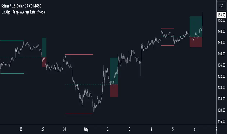
Range Average Retest Model [LuxAlgo]The Range Average Retest Model tool highlights setups from the range average retest entry model, a model using the retest of the average between two opposite swing points as an entry.
This tool uses long-term volatility coupled with user-defined multipliers to filter out swing areas and set take profit and stop loss levels for all trades.
Key features include:
Draw up to 165 swing areas and their associated trades
Filter out swing areas using Pivot Length , Selection Mode and Threshold parameters
Filter out trades with Maximum Distance and Minimum Distance parameters
Enable or disable swing areas and select default colors
Enable or disable overlapping trades and change the default colors for Take Profit and Stop Loss zones
🔶 USAGE
The "Range Average Retest Model" is an entry model that enters a position when the price retests the average made between two swing points. Users can determine the period of the detected swing points from the "Pivot Length" setting.
The conditions for long or short trades, regardless of whether the swing area is bullish or bearish, are as follows:
Long positions: the current bar close is below the swing area average and the last bar close was above it.
Short positions: the current bar close is above the swing area average price and the last bar close was below it.
Each trade is displayed on the chart with a line connecting it to its swing area highlighting the range average, a green area for the take profit, and a red area for the stop loss.
Both the Take Profit and Stop Loss levels are calculated by applying your own multiplier in the settings panel to the long-term volatility measure, in this case, the average true range over the last 200 bars.
Trades will remain open until they reach either the Stop Loss or Take Profit price levels.
🔹 Filtering Swing Areas
The daily chart of the Nasdaq-100 futures (NQ) with pivot length 2 and bullish selection mode: it only detects bullish swing areas, but they are smaller and more numerous.
Traders can manipulate the behavior of the swing areas from the settings panel.
The Selection mode will filter areas by bias: it will detect bullish areas, bearish areas, or both.
The Threshold parameter is applied to the long-term volatility to filter out areas where the average prices are too close together; the higher the value, the greater the difference between the average prices must be.
🔹 Trades
3-minute chart of the Nasdaq-100 futures (NQ) with pivot length 5, bearish selection mode maximum distance 4, and stop loss 2: many trades detected with very asymmetric risk/reward.
The behavior of the trades is also manipulated from the settings panel.
The maximum and minimum distance parameters specify the number of bars a trade must be away from a swing area.
The Take Profit and Stop Loss parameters are applied to the long-term volatility to obtain their respective price levels.
🔹 Overlapping Trades
Same chart as before, but with overlapping trades: messy, right?
By default the tool does not show overlapping trades, this allows for a cleaner chart.
In the settings panel traders can enable overlapping mode, in which case the tool will show all available trades.
Traders must be aware that the chart can be very crowded.
🔶 SETTINGS
🔹 Swings
Pivot Length: How many bars are used to confirm a swing point. The larger this parameter is, the larger and fewer swing areas will be detected.
Selection Mode: Swing area detection mode, detect only bullish swings, only bearish swings, or both.
Threshold: Swing area comparator. This threshold is multiplied by a measure of volatility (average true range over the last 200 bars), for a new swing area to be detected it must have an average level that is sufficiently distant from the average level of any untouched swing area, this parameter controls that distance.
🔹 Trades
Maximum distance: Maximum distance allowed between a swing area and a trade.
Minimum distance: Minimum distance allowed between a swing area and a trade.
Take profit: The size of the take profit - this threshold is multiplied by a measure of volatility (the average true range over the last 200 bars).
Stop loss: The size of the stop-loss: this threshold is multiplied by a measure of volatility (the average true range over the last 200 bars).
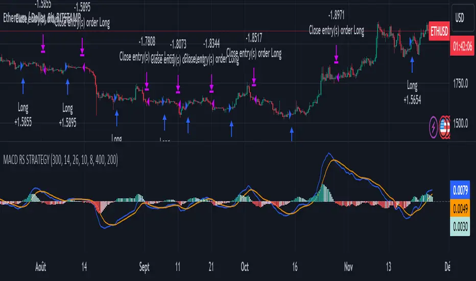
MACD of Relative Strenght StrategyMACD Relative Strenght Strategy :
INTRODUCTION :
This strategy is based on two well-known indicators: MACD and Relative Strenght (RS). By coupling them, we obtain powerful buy signals. In fact, the special feature of this strategy is that it creates an indicator from an indicator. Thus, we construct a MACD whose source is the value of the RS. The strategy only takes buy signals, ignoring SHORT signals as they are mostly losers. There's also a money management method enabling us to reinvest part of the profits or reduce the size of orders in the event of substantial losses.
RELATIVE STRENGHT :
RS is an indicator that measures the anomaly between momentum and the assumption of market efficiency. It is used by professionals and is one of the most robust indicators. The idea is to own assets that do better than average, based on their past performance. We calculate RS using this formula :
RS = close/highest_high(RS_Length)
Where highest_high(RS_Length) = highest value of the high over a user-defined time period (which is the RS_Length).
We can thus situate the current price in relation to its highest price over this user-defined period.
MACD (Moving Average Convergence - Divergence) :
This is one of the best-known indicators, measuring the distance between two exponential moving averages : one fast and one slower. A wide distance indicates fast momentum and vice versa. We'll plot the value of this distance and call this line macdline. The MACD uses a third moving average with a lower period than the first two. This last moving average will give a signal when it crosses the macdline. It is therefore constructed using the values of the macdline as its source.
It's important to note that the first two MAs are constructed using RS values as their source. So we've just built an indicator of an indicator. This kind of method is very powerful because it is rarely used and brings value to the strategy.
PARAMETERS :
RS Length : Relative Strength length i.e. the number of candles back to find the highest high and compare the current price with this high. Default is 300.
MACD Fast Length : Relative Strength fast EMA length used to plot the MACD. Default is 14.
MACD Slow Length : Relative Strength slow EMA length used to plot the MACD. Default is 26.
MACD Signal Smoothing : Macdline SMA length used to plot the MACD. Default is 10.
Max risk per trade (in %) : The maximum loss a trade can incur (in percentage of the trade value). Default is 8%.
Fixed Ratio : This is the amount of gain or loss at which the order quantity is changed. Default is 400, meaning that for each $400 gain or loss, the order size is increased or decreased by a user-selected amount.
Increasing Order Amount : This is the amount to be added to or subtracted from orders when the fixed ratio is reached. The default is $200, which means that for every $400 gain, $200 is reinvested in the strategy. On the other hand, for every $400 loss, the order size is reduced by $200.
Initial capital : $1000
Fees : Interactive Broker fees apply to this strategy. They are set at 0.18% of the trade value.
Slippage : 3 ticks or $0.03 per trade. Corresponds to the latency time between the moment the signal is received and the moment the order is executed by the broker.
Important : A bot has been used to test the different parameters and determine which ones maximize return while limiting drawdown. This strategy is the most optimal on BITSTAMP:ETHUSD in 8h timeframe with the parameters set by default.
ENTER RULES :
The entry rules are very simple : we open a long position when the MACD value turns positive. You are therefore LONG when the MACD is green.
EXIT RULES :
We exit a position (whether losing or winning) when the MACD becomes negative, i.e. turns red.
RISK MANAGEMENT :
This strategy can incur losses, so it's important to manage our risks well. If the position is losing and has incurred a loss of -8%, our stop loss is activated to limit losses.
MONEY MANAGEMENT :
The fixed ratio method was used to manage our gains and losses. For each gain of an amount equal to the value of the fixed ratio, we increase the order size by a value defined by the user in the "Increasing order amount" parameter. Similarly, each time we lose an amount equal to the value of the fixed ratio, we decrease the order size by the same user-defined value. This strategy increases both performance and drawdown.
Enjoy the strategy and don't forget to take the trade :)
Portfolio Backtester Engine█ OVERVIEW
Portfolio Backtester Engine (PBTE). This tool will allow you to backtest strategies across multiple securities at once. Allowing you to easier understand if your strategy is robust. If you are familiar with the PineCoders backtesting engine , then you will find this indicator pleasant to work with as it is an adaptation based on that work. Much of the functionality has been kept the same, or enhanced, with some minor adjustments I made on the account of creating a more subjectively intuitive tool.
█ HISTORY
The original purpose of the backtesting engine (`BTE`) was to bridge the gap between strategies and studies . Previously, strategies did not contain the ability to send alerts, but were necessary for backtesting. Studies on the other hand were necessary for sending alerts, but could not provide backtesting results . Often, traders would have to manage two separate Pine scripts to take advantage of each feature, this was less than ideal.
The `BTE` published by PineCoders offered a solution to this issue by generating backtesting results under the context of a study(). This allowed traders to backtest their strategy and simultaneously generate alerts for automated trading, thus eliminating the need for a separate strategy() script (though, even converting the engine to a strategy was made simple by the PineCoders!).
Fast forward a couple years and PineScript evolved beyond these issues and alerts were introduced into strategies. The BTE was not quite as necessary anymore, but is still extremely useful as it contains extra features and data not found under the strategy() context. Below is an excerpt of features contained by the BTE:
"""
More than `40` built-in strategies,
Customizable components,
Coupling with your own external indicator,
Simple conversion from Study to Strategy modes,
Post-Exit analysis to search for alternate trade outcomes,
Use of the Data Window to show detailed bar by bar trade information and global statistics, including some not provided by TV backtesting,
Plotting of reminders and generation of alerts on in-trade events.
"""
Before I go any further, I want to be clear that the BTE is STILL a good tool and it is STILL very useful. The Portfolio Backtesting Engine I am introducing is only a tangental advancement and not to be confused as a replacement, this tool would not have been possible without the `BTE`.
█ THE PROBLEM
Most strategies built in Pine are limited by one thing. Data. Backtesting should be a rigorous process and researchers should examine the performance of their strategy across all market regimes; that includes, bullish and bearish markets, ranging markets, low volatility and high volatility. Depending on your TV subscription The Pine Engine is limited to 5k-20k historical bars available for backtesting, which can often leave the strategy results wanting. As a general rule of thumb, strategies should be tested across a quantity of historical bars which will allow for at least 100 trades. In many cases, the lack of historical bars available for backtesting and frequency of the strategy signals produces less than 100 trades, rendering your strategy results inconclusive.
█ THE SOLUTION
In order to be confident that we have a robust strategy we must test it across all market regimes and we must have over 100 trades. To do this effectively, researchers can use the Portfolio Backtesting Engine (PBTE).
By testing a strategy across a carefully selected portfolio of securities, researchers can now gather 5k-20k historical bars per security! Currently, the PTBE allows up to 5 securities, which amounts to 25k-100k historical bars.
█ HOW TO USE
1 — Add the indicator to your chart.
• Confirm inputs. These will be the most important initial values which you can change later by clicking the gear icon ⚙ and opening up the settings of the indicator.
2 — Select a portfolio.
• You will want to spend some time carefully selecting a portfolio of securities.
• Each security should be uncorrelated.
• The entire portfolio should contain a mix of different market regimes.
You should understand that strategies generally take advantage of one particular type of market regime. (trending, ranging, low/high volatility)
For example, the default RSI strategy is typically advantageous during ranging markets, whereas a typical moving average crossover strategy is advantageous in trending markets.
If you were to use the standard RSI strategy during a trending market, you might be selling when you should be buying.
Similarily, if you use an SMA crossover during a ranging market, you will find that the MA's may produce many false signals.
Even if you build a strategy that is designed to be used only in a trending market, it is still best to select a portfolio of all market regimes
as you will be able to test how your strategy will perform when the market does something unexpected.
3 — Test a built-in strategy or add your own.
• Navigate to gear icon ⚙ (settings) of strategy.
• Choose your options.
• Select a Main Entry Strat and Alternate Entry Strat .
• If you want to add your own strategy, you will need to modify the source code and follow the built-in example.
• You will only need to generate (buy 1 / sell -1/ neutral 0) signals.
• Select a Filter , by default these are all off.
• Select an Entry Stop - This will be your stop loss placed at the trade entry.
• Select Pyamiding - This will allow you to stack positions. By default this is off.
• Select Hard Exits - You can also think of these as Take Profits.
• Let the strategy run and take note of the display tables results.
• Portfolio - Shows each security.
• The strategy runs on each asset in your portfolio.
• The initial capital is equally distributed across each security.
So if you have 5 securities and a starting capital of 100,000$ then each security will run the strategy starting with 20,000$
The total row will aggregate the results on a bar by bar basis showing the total results of your initial capital.
• Net Profit (NP) - Shows profitability.
• Number of Trades (#T) - Shows # of trades taken during backtesting period.
• Typically will want to see this number greater than 100 on the "Total" row.
• Average Trade Length (ATL) - Shows average # of days in a trade.
• Maximum Drawdown (MD ) - Max peak-to-valley equity drawdown during backtesting period.
• This number defines the minimum amount of capital required to trade the system.
• Typically, this shouldn’t be lower than 34% and we will want to allow for at least 50% beyond this number.
• Maximum Loss (ML) - Shows largest loss experienced on a per-trade basis.
• Normally, don’t want to exceed more than 1-2 % of equity.
• Maximum Drawdown Duration (MDD) - The longest duration of a drawdown in equity prior to a new equity peak.
• This number is important to help us psychologically understand how long we can expect to wait for a new peak in account equity.
• Maximum Consecutive Losses (MCL) - The max consecutive losses endured throughout the backtesting period.
• Another important metric for trader psychology, this will help you understand how many losses you should be prepared to handle.
• Profit to Maximum Drawdown (P:MD) - A ratio for the average profit to the maximum drawdown.
• The higher the ratio is, the better. Large profits and small losses contribute to a good PMD.
• This metric allows us to examine the profit with respect to risk.
• Profit Loss Ratio (P:L) - Average profit over the average loss.
• Typically this number should be higher in trend following systems.
• Mean reversion systems show lower values, but compensate with a better win %.
• Percent Winners (% W) - The percentage of winning trades.
• Trend systems will usually have lower win percentages, since statistically the market is only trending roughly 30% of the time.
• Mean reversion systems typically should have a high % W.
• Time Percentage (Time %) - The amount of time that the system has an open position.
• The more time you are in the market, the more you are exposed to market risk, not to mention you could be using that money for something else right?
• Return on Investment (ROI) - Your Net Profit over your initial investment, represented as a percentage.
• You want this number to be positive and high.
• Open Profit (OP) - If the strategy has any open positions, the floating value will be represented here.
• Trading Days (TD) - An important metric showing how many days the strategy was active.
• This is good to know and will be valuable in understanding how long you will need to run this strategy in order to achieve results.
█ FEATURES
These are additional features that extend the original `BTE` features.
- Portfolio backtesting.
- Color coded performance results.
- Circuit Breakers that will stop trading.
- Position reversals on exit. (Simulating the function of always in the market. Similar to strategy.entry functionality)
- Whipsaw Filter
- Moving Average Filter
- Minimum Change Filter
- % Gain Equity Exit
- Popular strategies, (MACD, MA cross, supertrend)
Below are features that were excluded from the original `BTE`
- 2 stage in-trade stops with kick-in rules (This was a subjective decision to remove. I found it to be complex and thwarted my use of the `BTE` for some time.)
- Simple conversion from Study to Strategy modes. (Not possible with multiple securities)
- Coupling with your own external indicator (Not really practical to use with multiple securities, but could be used if signals were generated based on some indicator which was not based on the current chart)
- Use of the Data Window to show detailed bar by bar trade information and global statistics.
- Post Exit Analysis.
- Plotting of reminders and generation of alerts on in-trade events.
- Alerts (These may be added in the future by request when I find the time.)
█ THANKS
The whole PineCoders team for all their shared knowledge and original publication of the BTE and Richard Weismann for his ideas on building robust strategies.
═════════════════════════════════════════════════════════════════════════

Bollinger Bands Strategy with Intraday Intensity IndexFor Educational Purposes. Results can differ on different markets and can fail at any time. Profit is not guaranteed.
This only works in a few markets and in certain situations. Changing the settings can give better or worse results for other markets.
This is a mean reversion strategy based on Bollinger Bands and the Intraday Intensity Index (a volume indicator). John Bollinger mentions that the Intraday Intensity Index can be used with Bollinger Bands and is one of the top indicators he recommends in his book. It seems he prefers it over the other volume indicators that he compares to for some reason. III looks a lot like Chaikin Money Flow but without the denominator in that calculation. On the default settings of the BBs, the III helps give off better entry signals. John Bollinger however is vague on how to use the BBs and it's hard to say if one should enter when it is below/above the bands or when the price crosses them. I find that with many indicators and strategies it's best to wait for a confirmation of some sort, in this case by waiting for some crossover of a band. Like most mean reversion strategies, the exit is very loose if using BBs alone. Usually the plan to exit is when the price finally reverts back to the mean or in this case the middle band. This can potentially lead to huge drawdowns and/or losses. Mean reversion strategies can have high win/loss ratios but can still end up unprofitable because of the huge losses that can occur. These drawdowns/losses that mean reversion strategies suffer from can potentially eat away at a large chunk of all that was previously made or perhaps up to all of it in the worst cases, can occur weeks or perhaps up to months after being profitable trading such a strategy, and will take a while and several trades to make it all back or keep a profitable track record. It is important to have a stop loss, trailing stop, or some sort of stop plan with these types of strategies. For this one, in addition to exiting the trade when price reverts to the middle band, I included a time-based stop plan that exits with a gain or with a loss to avoid potentially large losses, and to exit after only a few periods after taking the trade if in profit instead of waiting for the price to revert back to the mean.
NeuraEdge ORB - Opening Range Breakout IndicatorOVERVIEW
NeuraEdge ORB is an open-source Opening Range Breakout indicator that automates the classic 15-minute ORB strategy. The indicator tracks the first 15 minutes of market action (9:30-9:45 AM ET), identifies breakouts above or below this range, and generates trading signals with automated stop loss and take profit calculations.
The Opening Range Breakout concept is based on the observation that the initial price action after market open often establishes directional bias for the trading session, as institutional order flow and overnight gap reactions manifest during this window.
CORE METHODOLOGY
Opening Range Construction:
The indicator uses session-based time detection to identify the 9:30-9:45 AM Eastern Time window. During this period, it tracks the highest high and lowest low to establish the opening range boundaries. The range is marked complete when the 15-minute window closes.
Calculation process:
OR High = Maximum high value during the 15-minute window
OR Low = Minimum low value during the 15-minute window
OR Midpoint = (OR High + OR Low) / 2
Range Size = OR High - OR Low (compared to 14-period ATR for context)
Breakout Detection:
The indicator identifies breakouts using close-price confirmation to reduce false signals from wicks:
Bullish breakout: Close above OR High (with previous close at or below OR High)
Bearish breakout: Close below OR Low (with previous close at or above OR Low)
The indicator tracks whether each direction has already broken to prevent duplicate signals on the same range.
Entry Type Logic:
Two entry methodologies are supported:
Breakout Mode - Signals immediately upon range break. Enters on the breakout bar when close confirms direction.
Retest Mode - Waits for price to break the range, then pullback to touch the range level before entering. Cancels if price moves too far beyond midpoint. This provides better entry prices with tighter stop losses.
Volume Confirmation:
Optional volume filter compares current bar volume to 20-period simple moving average. Requires volume > 1.2x average to validate breakout strength and filter low-conviction moves.
Fair Value Gap (FVG) Integration:
Optional confluence filter that checks for unfilled FVG in the breakout direction:
Bullish FVG detected when: current bar's low > two bars ago high (creating gap)
Bearish FVG detected when: current bar's high < two bars ago low (creating gap)
Minimum FVG size: 0.3x ATR to filter noise
FVG considered filled when price retraces to gap midpoint
Signals only generate when an unfilled FVG exists in the breakout direction, adding institutional order flow confluence.
Risk Management Calculations:
Three stop loss placement methods:
Opposite Side - SL at opposite end of opening range (classic ORB approach)
Midpoint - SL at range midpoint (tighter risk, lower reward potential)
ATR Based - SL at 1.5x ATR from entry (adaptive to volatility)
Take profit calculated as: Entry ± (Entry - Stop Loss) × Risk:Reward Ratio
Default 1.5:1 R:R ratio, adjustable from 1.0 to 5.0.
Performance Tracking:
The indicator maintains a trade history using Pine Script's type system:
Records entry price, stop loss, take profit, and direction for each signal
Tracks outcome when price hits stop loss or take profit levels
Auto-closes after 80 bars if neither level hit
Calculates rolling win rate from last 50 trades maximum
Displays W/L record in real-time dashboard
VISUAL COMPONENTS
Opening Range Box:
Semi-transparent blue box drawn from range start bar to current bar + 20, showing the established range boundaries visually.
Range Levels:
Green line at OR High (potential long entry level)
Red line at OR Low (potential short entry level)
Gray dotted line at OR Midpoint (reference level)
All lines extend 50 bars forward for anticipation.
Trade Signals:
Green up arrow with "LONG ORB Break" label below price
Red down arrow with "SHORT ORB Break" label above price
Dashed lines showing SL and TP levels extending 30 bars
Small labels marking SL and TP endpoints
Real-Time Dashboard:
Top-right panel displaying:
OR formation status (Forming / Complete / Waiting)
Current OR High, Low, and Range size (with ATR multiple)
Breakout status (Long / Short / None)
Volume status (High / Normal)
FVG presence (Bull / Bear / None)
Entry settings (Breakout/Retest, R:R, SL type)
Win rate percentage and W/L record
PRACTICAL APPLICATION
Ideal Market Conditions:
Liquid instruments: SPY, QQQ, IWM, high-volume stocks
Recommended timeframes: 1-minute or 5-minute charts for precise entries
Most effective during trending days with clear directional bias
Range size between 0.5-1.5x ATR typically provides best risk:reward
Usage Workflow:
Apply indicator at market open (9:30 AM ET)
Observe range formation during first 15 minutes
Wait for "Complete" status in dashboard
Monitor for breakout signals with volume/FVG confirmation
Enter on signal, place stop loss and take profit as marked
Avoid taking opposing signals on same day (trend following approach)
Retest vs Breakout Selection:
Use Breakout mode on high-momentum days with strong overnight gaps
Use Retest mode on slower days or when seeking better entry prices
Retest mode reduces signal frequency but improves entry quality
Time-of-Day Considerations:
The indicator includes a trading cutoff setting (default 3:00 PM ET) to avoid late-day chop and reduced liquidity. First-hour breakouts (10:00-11:00 AM) historically show strongest follow-through.
SETTINGS & CUSTOMIZATION
Display Options:
Toggle signals, opening range box, and dashboard independently
Clean visual design to reduce chart clutter
Opening Range Settings:
Opening range duration (5-60 minutes in 5-minute increments)
Default 15 minutes aligns with classic ORB methodology
Trading cutoff hour (10-16, representing 10:00 AM - 4:00 PM ET)
Entry Configuration:
Entry type (Breakout / Retest)
Volume confirmation toggle (requires 1.2x average volume)
FVG confluence toggle (requires unfilled gap in breakout direction)
Risk Management:
Stop loss placement (Opposite Side / Midpoint / ATR Based)
Risk:reward ratio (1.0 - 5.0, default 1.5)
Future: Trail stop after partial TP (currently placeholder)
Alert System:
Five alert conditions available:
Opening Range Complete
ORB Long Signal
ORB Short Signal
Breakout Up (range broken, regardless of signal)
Breakout Down (range broken, regardless of signal)
BEST PRACTICES
Recommended Usage:
Focus on highly liquid instruments with tight spreads
Use 1-5 minute charts for entry precision
Respect calculated stop losses (range defines maximum risk)
Typically 1-2 quality setups per day maximum
Consider overall market trend (SPY/QQQ direction)
Risk Considerations:
Very small ranges (< 0.3x ATR) prone to false breakouts
Very large ranges (> 2x ATR) may indicate gap day requiring adjusted expectations
Low volume breakouts fail more frequently
Avoid trading both directions on same day (pick strongest setup)
IMPORTANT DISCLOSURES
This indicator is provided free and open-source for educational purposes. The Opening Range Breakout strategy is a well-documented public domain trading concept. This implementation adds automation, visual clarity, and optional confluence filters.
No indicator guarantees profitable trades. Past performance does not predict future results. Traders are responsible for their own trading decisions and risk management. Always use appropriate position sizing and never risk more than you can afford to lose.

CryptoFlux Dynamo [JOAT]CryptoFlux Dynamo: Velocity Scalping Strategy
WHAT THIS STRATEGY IS
CryptoFlux Dynamo is an open-source Pine Script v6 strategy designed for momentum-based scalping on cryptocurrency perpetual futures. It combines multiple technical analysis methods into a unified system that adapts its behavior based on current market volatility conditions.
This script is published open-source so you can read, understand, and modify the complete logic. The description below explains everything the strategy does so that traders who cannot read Pine Script can fully understand how it works before using it.
HOW THIS STRATEGY IS ORIGINAL AND WHY THE INDICATORS ARE COMBINED
This strategy uses well-known indicators (MACD, EMA, RSI, MFI, Bollinger Bands, Keltner Channels, ATR). The originality is not in the individual indicators themselves, but in the specific way they are integrated into a regime-adaptive system. Here is the detailed justification for why these components are combined and how they work together:
The Problem Being Solved:
Standard indicator-based strategies use fixed thresholds. For example, a typical MACD strategy might enter when the histogram crosses above zero. However, in cryptocurrency markets, volatility changes dramatically throughout the day and week. A MACD crossover during a low-volatility consolidation period has very different implications than the same crossover during a high-volatility trending period. Using the same entry thresholds and stop distances in both conditions leads to either:
Too many false signals during consolidation (if thresholds are loose)
Missing valid opportunities during expansion (if thresholds are tight)
Stops that are too tight during volatility spikes (causing premature exits)
Stops that are too wide during compression (giving back profits)
The Solution Approach:
This strategy first classifies the current volatility regime using normalized ATR (ATR as a percentage of price), then dynamically adjusts ALL other parameters based on that classification. This creates a context-aware system rather than a static threshold comparison.
How Each Component Contributes to the System:
ATR-Based Regime Classification (The Foundation)
The strategy calculates ATR over 21 periods, smooths it with a 13-period EMA to reduce noise from wicks, then divides by price to get a normalized percentage. This ATR% is classified into three regimes:
- Compression (ATR% < 0.8%): Market is consolidating, breakouts are more likely but false signals are common
- Expansion (ATR% 0.8% - 1.6%): Normal trending conditions
- Velocity (ATR% > 1.6%): High volatility, larger moves but also larger adverse excursions
This regime classification then controls stop distances, profit targets, trailing stop offsets, and signal strength requirements. The regime acts as a "meta-parameter" that tunes the entire system.
EMA Ribbon (8/21/34) - Trend Structure Detection
The three EMAs establish trend direction and structure. When EMA 8 > EMA 21 > EMA 34, the trend structure is bullish. The slope of the middle EMA (21) is calculated over 8 bars and converted to degrees using arctangent. This slope measurement quantifies trend strength, not just direction.
Why these specific periods? The 8/21/34 sequence follows Fibonacci-like spacing and provides good separation on 5-minute cryptocurrency charts. The fast EMA (8) responds to immediate price action, the mid EMA (21) represents the short-term trend, and the slow EMA (34) acts as a trend filter.
The EMA ribbon works with the regime classification: during compression regimes, the strategy requires stronger ribbon alignment before entry because false breakouts are more common.
MACD (8/21/5) - Momentum Measurement
The MACD uses faster parameters (8/21/5) than the standard (12/26/9) because cryptocurrency markets move faster than traditional markets. The histogram is smoothed with a 5-period EMA to reduce noise.
The key innovation is the adaptive histogram baseline. Instead of using a fixed threshold, the strategy calculates a rolling baseline from the smoothed absolute histogram value, then multiplies by a sensitivity factor (1.15). This means the threshold for "significant momentum" automatically adjusts based on recent momentum levels.
The MACD works with the regime classification: during velocity regimes, the histogram baseline is effectively higher because recent momentum has been stronger, preventing entries on relatively weak momentum.
RSI (21 period) and MFI (21 period) - Independent Momentum Confirmation
RSI measures momentum using price changes only. MFI (Money Flow Index) measures momentum using price AND volume. By requiring both to confirm, the strategy filters out price moves that lack volume support.
The 21-period length is longer than typical (14) to reduce noise on 5-minute charts. The trigger threshold (55 for longs, 45 for shorts) is slightly offset from 50 to require momentum in the trade direction, not just neutral readings.
These indicators work together: a signal requires RSI > 55 AND MFI > 55 for longs. This dual confirmation reduces false signals from price manipulation or low-volume moves.
Bollinger Bands (1.5 mult) and Keltner Channels (1.8 mult) - Squeeze Detection
When Bollinger Bands contract inside Keltner Channels, volatility is compressing and a breakout is likely. This is the "squeeze" condition. When the bands expand back outside the channels, the squeeze "releases."
The strategy uses a 1.5 multiplier for Bollinger Bands (tighter than standard 2.0) and 1.8 for Keltner Channels. These values were chosen to identify meaningful squeezes on 5-minute cryptocurrency charts without triggering too frequently.
The squeeze detection works with the regime classification: squeeze releases during compression regimes receive additional signal strength points because breakouts from consolidation are more significant.
Volume Impulse Detection - Institutional Participation Filter
The strategy calculates a volume baseline (34-period SMA) and standard deviation. A "volume impulse" is detected when current volume exceeds the baseline by 1.15x OR when the volume z-score exceeds 0.5.
This filter ensures entries occur when there is meaningful market participation, not during low-volume periods where price moves are less reliable.
Volume impulse is required for all entries and adds points to the composite signal strength score.
Cycle Oscillator - Trend Alignment Filter
The strategy calculates a 55-period EMA as a cycle basis, then measures price deviation from this basis as a percentage. When price is more than 0.15% above the cycle basis, the cycle is bullish. When more than 0.15% below, the cycle is bearish.
This filter prevents counter-trend entries. Long signals require bullish cycle alignment; short signals require bearish cycle alignment.
BTC Dominance Filter (Optional) - Market Regime Filter
The strategy can optionally use BTC.D (Bitcoin Dominance) as a market regime filter. When BTC dominance is rising (slope > 0.12), the market is in "risk-off" mode and long entries on altcoins are filtered. When dominance is falling (slope < -0.12), short entries are filtered.
This filter is optional because the BTC.D data feed may lag during low-liquidity periods.
How The Components Work Together (The Mashup Justification):
The strategy uses a composite scoring system where each signal pathway contributes points:
Trend Break pathway (30 points): Requires EMA ribbon alignment + positive slope + price breaks above recent structure high
Momentum Surge pathway (30 points): Requires MACD histogram > adaptive baseline + MACD line > signal + RSI > 55 + MFI > 55 + volume impulse
Squeeze Release pathway (25 points): Requires BB inside KC (squeeze) then release + momentum bias + histogram confirmation
Micro Pullback pathway (15 points): Requires shallow retracement to fast EMA within established trend + histogram confirmation + volume impulse
Additional modifiers:
+5 points if volume impulse is present, -5 if absent
+5 points in velocity regime, -2 in compression regime
+5 points if cycle is aligned, -5 if counter-trend
A trade only executes when the composite score reaches the minimum threshold (default 55) AND all filters agree (session, cycle bias, BTC dominance if enabled).
This scoring system is the core innovation: instead of requiring ALL conditions to be true (which would generate very few signals) or ANY condition to be true (which would generate too many false signals), the strategy requires ENOUGH conditions to be true, with different conditions contributing different weights based on their reliability.
HOW THE STRATEGY CALCULATES ENTRIES AND EXITS
Entry Logic:
1. Calculate current volatility regime from ATR%
2. Calculate all indicator values (MACD, EMA, RSI, MFI, squeeze, volume)
3. Evaluate each signal pathway and sum points
4. Check all filters (session, cycle, dominance, kill switch)
5. If composite score >= 55 AND all filters pass, generate entry signal
6. Calculate position size based on risk per trade and regime-adjusted stop distance
7. Execute entry with regime name as comment
Position Sizing Formula:
RiskCapital = Equity * (0.65 / 100)
StopDistance = ATR * StopMultiplier(regime)
RawQuantity = RiskCapital / StopDistance
MaxQuantity = Equity * (12 / 100) / Price
Quantity = min(RawQuantity, MaxQuantity)
Quantity = round(Quantity / 0.001) * 0.001
This ensures each trade risks approximately 0.65% of equity regardless of volatility, while capping total exposure at 12% of equity.
Stop Loss Calculation:
Stop distance is ATR multiplied by a regime-specific multiplier:
Compression regime: 1.05x ATR (tighter stops because moves are smaller)
Expansion regime: 1.55x ATR (standard stops)
Velocity regime: 2.1x ATR (wider stops to avoid premature exits during volatility)
Take Profit Calculation:
Target distance is ATR multiplied by regime-specific multiplier and base risk/reward:
Compression regime: 1.6x ATR * 1.8 base R:R * 0.9 regime bonus = approximately 2.6x ATR
Expansion regime: 2.05x ATR * 1.8 base R:R * 1.0 regime bonus = approximately 3.7x ATR
Velocity regime: 2.8x ATR * 1.8 base R:R * 1.15 regime bonus = approximately 5.8x ATR
Trailing Stop Logic:
When adaptive trailing is enabled, the strategy calculates a trailing offset based on ATR and regime:
Compression regime: 1.1x base offset (looser trailing to avoid noise)
Expansion regime: 1.0x base offset (standard)
Velocity regime: 0.8x base offset (tighter trailing to lock in profits during fast moves)
The trailing stop only activates when it would be tighter than the initial stop.
Momentum Fail-Safe Exits:
The strategy closes positions early if momentum reverses:
Long positions close if MACD histogram turns negative OR EMA ribbon structure breaks (fast EMA crosses below mid EMA)
Short positions close if MACD histogram turns positive OR EMA ribbon structure breaks
This prevents holding through momentum reversals even if stop loss hasn't been hit.
Kill Switch:
If maximum drawdown exceeds 6.5%, the strategy disables new entries until manually reset. This prevents continued trading during adverse conditions.
HOW TO USE THIS STRATEGY
Step 1: Apply to Chart
Use a 5-minute chart of a high-liquidity cryptocurrency perpetual (BTC/USDT, ETH/USDT recommended)
Ensure at least 200 bars of history are loaded for indicator stabilization
Use standard candlestick charts only (not Heikin Ashi, Renko, or other non-standard types)
Step 2: Understand the Visual Elements
EMA Ribbon: Three lines (8/21/34 periods) showing trend structure. Bullish when stacked upward, bearish when stacked downward.
Background Color: Shows current volatility regime
- Indigo/dark blue = Compression (low volatility)
- Purple = Expansion (normal volatility)
- Magenta/pink = Velocity (high volatility)
Bar Colors: Reflect signal strength divergence. Brighter colors indicate stronger directional bias.
Triangle Markers: Entry signals. Up triangles below bars = long entry. Down triangles above bars = short entry.
Dashboard (top-right): Real-time display of regime, ATR%, signal strengths, position status, stops, targets, and risk metrics.
Step 3: Interpret the Dashboard
Regime: Current volatility classification (Compression/Expansion/Velocity)
ATR%: Normalized volatility as percentage of price
Long/Short Strength: Current composite signal scores (0-100)
Cycle Osc: Price deviation from 55-period EMA as percentage
Dominance: BTC.D slope and filter status
Position: Current position direction or "Flat"
Stop/Target: Current stop loss and take profit levels
Kill Switch: Status of drawdown protection
Volume Z: Current volume z-score
Impulse: Whether volume impulse condition is met
Step 4: Adjust Parameters for Your Needs
For more conservative trading: Increase "Minimum Composite Signal Strength" to 65 or higher
For more aggressive trading: Decrease to 50 (but expect more false signals)
For higher timeframes (15m+): Increase "Structure Break Window" to 12-15, increase "RSI Momentum Trigger" to 58
For lower liquidity pairs: Increase "Volume Impulse Multiplier" to 1.3, increase slippage in strategy properties
To disable short selling: Uncheck "Enable Short Structure"
To disable BTC dominance filter: Uncheck "BTC Dominance Confirmation"
STRATEGY PROPERTIES (BACKTEST SETTINGS)
These are the exact settings used in the strategy's Properties dialog box. You must use these same settings when evaluating the backtest results shown in the publication:
Initial Capital: $100,000
Justification: This amount is higher than typical retail accounts. I chose this value to demonstrate percentage-based returns that scale proportionally. The strategy uses percentage-based position sizing (0.65% risk per trade), so a $10,000 account would see the same percentage returns with 10x smaller position sizes. The absolute dollar amounts in the backtest should be interpreted as percentages of capital.
Commission: 0.04% (commission_value = 0.04)
Justification: This reflects typical perpetual futures exchange fees. Major exchanges charge between 0.02% (maker) and 0.075% (taker). The 0.04% value is a reasonable middle estimate. If your exchange charges different fees, adjust this value accordingly. Higher fees will reduce net profitability.
Slippage: 1 tick
Justification: This is conservative for liquid pairs like BTC/USDT on major exchanges during normal conditions. For less liquid altcoins or during high volatility, actual slippage may be higher. If you trade less liquid pairs, increase this value to 2-3 ticks for more realistic results.
Pyramiding: 1
Justification: No position stacking. The strategy holds only one position at a time. This simplifies risk management and prevents overexposure.
calc_on_every_tick: true
Justification: The strategy evaluates on every price update, not just bar close. This is necessary for scalping timeframes where waiting for bar close would miss opportunities. Note that this setting means backtest results may differ slightly from bar-close-only evaluation.
calc_on_order_fills: true
Justification: The strategy recalculates immediately after order fills for faster response to position changes.
RISK PER TRADE JUSTIFICATION
The default risk per trade is 0.65% of equity. This is well within the TradingView guideline that "risking more than 5-10% on a trade is not typically considered viable."
With the 12% maximum exposure cap, even if the strategy takes multiple consecutive losses, the total risk remains manageable. The kill switch at 6.5% drawdown provides additional protection by halting new entries during adverse conditions.
The position sizing formula ensures that stop distance (which varies by regime) is accounted for, so actual risk per trade remains approximately 0.65% regardless of volatility conditions.
SAMPLE SIZE CONSIDERATIONS
For statistically meaningful backtest results, you should select a dataset that generates at least 100 trades. On 5-minute BTC/USDT charts, this typically requires:
2-3 months of data during normal market conditions
1-2 months during high-volatility periods
3-4 months during low-volatility consolidation periods
The strategy's selectivity (requiring 55+ composite score plus all filters) means it generates fewer signals than less filtered approaches. If your backtest shows fewer than 100 trades, extend the date range or reduce the minimum signal strength threshold.
Fewer than 100 trades produces statistically unreliable results. Win rate, profit factor, and other metrics can vary significantly with small sample sizes.
STRATEGY DESIGN COMPROMISES AND LIMITATIONS
Every strategy involves trade-offs. Here are the compromises made in this design and the limitations you should understand:
Selectivity vs. Opportunity Trade-off
The 55-point minimum threshold filters many potential trades. This reduces false signals but also misses valid setups that don't meet all criteria. Lowering the threshold increases trade frequency but decreases win rate. There is no "correct" threshold; it depends on your preference for fewer higher-quality signals vs. more signals with lower individual quality.
Regime Classification Lag
The ATR-based regime detection uses historical data (21 periods + 13-period smoothing). It cannot predict sudden volatility spikes. During flash crashes or black swan events, the strategy may be classified in the wrong regime for several bars before the classification updates. This is an inherent limitation of any lagging indicator.
Indicator Parameter Sensitivity
The default parameters (MACD 8/21/5, EMA 8/21/34, RSI 21, etc.) are tuned for BTC/ETH perpetuals on 5-minute charts during 2024 market conditions. Different assets, timeframes, or market regimes may require different parameters. There is no guarantee that parameters optimized on historical data will perform similarly in the future.
BTC Dominance Filter Limitations
The CRYPTOCAP:BTC.D data feed may lag during low-liquidity periods or weekends. The dominance slope calculation uses a 5-bar SMA, adding additional delay. If you notice the filter behaving unexpectedly, consider disabling it.
Backtest vs. Live Execution Differences
TradingView backtesting does not replicate actual broker execution. Key differences:
Backtests assume perfect fills at calculated prices; real execution involves order book depth, latency, and partial fills
The calc_on_every_tick setting improves backtest realism but still cannot capture sub-bar price action or order book dynamics
Commission and slippage settings are estimates; actual costs vary by exchange, time of day, and market conditions
Funding rates on perpetual futures are not modeled in backtests and can significantly impact profitability over time
Exchange-specific limitations (position limits, liquidation mechanics, order types) are not modeled
Market Condition Dependencies
This strategy is designed for trending and breakout conditions. During extended sideways consolidation with no clear direction, the strategy may generate few signals or experience whipsaws. No strategy performs well in all market conditions.
Cryptocurrency-Specific Risks
Cryptocurrency markets operate 24/7 without session boundaries. This means:
No natural "overnight" risk reduction
Volatility can spike at any time
Liquidity varies significantly by time of day
Exchange outages or issues can occur at any time
WHAT THIS STRATEGY DOES NOT DO
To be straightforward about limitations:
This strategy does not guarantee profits. Past backtest performance does not indicate future results.
This strategy does not predict the future. It reacts to current conditions based on historical patterns.
This strategy does not account for funding rates, which can significantly impact perpetual futures profitability.
This strategy does not model exchange-specific execution issues (partial fills, requotes, outages).
This strategy does not adapt to fundamental news events or black swan scenarios.
This strategy is not optimized for all market conditions. It may underperform during extended consolidation.
IMPORTANT RISK WARNINGS
Past performance does not guarantee future results. The backtest results shown reflect specific historical market conditions and parameter settings. Markets change constantly, and strategies that performed well historically may underperform or lose money in the future. A single backtest run does not constitute proof of future profitability.
Trading involves substantial risk of loss. Cryptocurrency derivatives are highly volatile instruments. You can lose your entire investment. Only trade with capital you can afford to lose completely.
This is not financial advice. This strategy is provided for educational and informational purposes only. It does not constitute investment advice, trading recommendations, or any form of financial guidance. The author is not a licensed financial advisor.
You are responsible for your own decisions. Before using this strategy with real capital:
Thoroughly understand the code and logic by reading the open-source implementation
Forward test with paper trading or very small positions for an extended period
Verify that commission, slippage, and execution assumptions match your actual trading environment
Understand that live results will differ from backtest results
Consider consulting with a qualified financial advisor
No guarantees or warranties. This strategy is provided "as is" without any guarantees of profitability, accuracy, or suitability for any purpose. The author is not responsible for any losses incurred from using this strategy.
OPEN-SOURCE CODE STRUCTURE
The strategy code is organized into these sections for readability:
Configuration Architecture: Input parameters organized into logical groups (Core Controls, Optimization Constants, Regime Intelligence, Signal Pathways, Risk Architecture, Visualization)
Helper Functions: calcQty() for position sizing, clamp01() and normalize() for value normalization, calcMFI() for Money Flow Index calculation
Core Indicator Engine: EMA ribbon, ATR and regime classification, MACD with adaptive baseline, RSI, MFI, volume analytics, cycle oscillator, BTC dominance filter, squeeze detection
Signal Pathway Logic: Trend break, momentum surge, squeeze release, micro pullback pathways with composite scoring
Entry/Exit Orchestration: Signal filtering, position sizing, entry execution, stop/target calculation, trailing stop logic, momentum fail-safe exits
Visualization Layer: EMA plots, regime background, bar coloring, signal labels, dashboard table
You can read and modify any part of the code. Understanding the logic before deployment is strongly recommended.
- Made with passion by officialjackofalltrades

Latent Energy Reactor [The_lurker]Latent Energy Reactor | مفاعل الطاقة الكامنة
═════════════════════════════════════════════════════════════
🔬 THE PHILOSOPHY
═════════════════════════════════════════════════════════════
Markets operate in cycles of compression and expansion. Before every significant price movement, there exists a period where buyers and sellers reach a temporary equilibrium — a consolidation zone where energy accumulates like pressure building in a reactor.
The Latent Energy Reactor was designed to identify these critical zones, measure the energy building within them, and predict the direction of the inevitable breakout.
This indicator transforms the abstract concept of "market energy" into a quantifiable, visual system that traders can use to anticipate high-probability breakout opportunities.
═════════════════════════════════════════════════════════════
🎯 THE THREE BOX STATES
═════════════════════════════════════════════════════════════
Understanding the three box states is crucial for proper interpretation:
📦 STATE 1: ACTIVE ZONE (GRAY BOX)
─────────────────────────────────────
Visual Characteristics:
• Color: Gray/Neutral with 3D depth effect
• Extends to the right edge of the chart (future projection)
• Contains pressure lines (dotted horizontal lines inside)
• Displays gravity center line (dashed line showing volume-weighted center)
• Energy progress bar beneath the box
• Real-time information panel appears on screen
What It Means:
The gray box represents a LIVE consolidation zone currently forming. Price is contained within the boundaries, and energy is actively accumulating. This is the "waiting phase" where the reactor is charging.
What to Watch:
• Energy percentage climbing toward critical levels (80%+)
• Gravity center position (upper half = bullish bias, lower half = bearish bias)
• Top and bottom rejection counts in the information panel
• Phase progression (Forming → Growth → Mature → Exhaustion)
Trading Approach:
Do NOT trade inside the gray box. This is the preparation phase. Monitor the energy levels and predicted direction, but wait for confirmation.
📦 STATE 2: BULLISH BREAKOUT BOX (GREEN BOX)
─────────────────────────────────────────────
Visual Characteristics:
• Color: Green with 3D depth effect
• Box boundaries are now fixed (no longer extending right)
• Displays "BUY" text centered inside the box
• Stop Loss line appears below the box (orange)
• Three Take Profit lines appear above (teal/cyan)
• Entry line at the box's upper boundary (white dashed)
What It Means:
The green box indicates a CONFIRMED bullish breakout. Price has broken above the consolidation zone's upper boundary, releasing the accumulated energy upward.
Automatic Calculations Displayed:
• Entry Price: Upper boundary of the box
• Stop Loss: Lower boundary minus ATR buffer
• TP1: Entry + (Risk × 1.0) — 1:1 reward ratio
• TP2: Entry + (Risk × 1.5) — 1.5:1 reward ratio
• TP3: Entry + (Risk × 2.0) — 2:1 reward ratio
Trading Approach:
Consider long positions with the displayed SL/TP levels as guidelines. The higher the energy level and breakout quality score were before the breakout, the more reliable the signal.
📦 STATE 3: BEARISH BREAKOUT BOX (RED BOX)
──────────────────────────────────────────
Visual Characteristics:
• Color: Red with 3D depth effect
• Box boundaries are now fixed
• Displays "SELL" text centered inside the box
• Stop Loss line appears above the box (orange)
• Three Take Profit lines appear below (teal/cyan)
• Entry line at the box's lower boundary (white dashed)
What It Means:
The red box indicates a CONFIRMED bearish breakout. Price has broken below the consolidation zone's lower boundary, releasing the accumulated energy downward.
Automatic Calculations Displayed:
• Entry Price: Lower boundary of the box
• Stop Loss: Upper boundary plus ATR buffer
• TP1: Entry - (Risk × 1.0) — 1:1 reward ratio
• TP2: Entry - (Risk × 1.5) — 1.5:1 reward ratio
• TP3: Entry - (Risk × 2.0) — 2:1 reward ratio
Trading Approach:
Consider short positions with the displayed SL/TP levels as guidelines. Stronger setups have higher pre-breakout energy and quality scores.
═════════════════════════════════════════════════════════════
⚛️ THE ENERGY CALCULATION SYSTEM
═════════════════════════════════════════════════════════════
The energy percentage (0-100%) is calculated using four factors:
Compression Score (up to 40 points)
Measures how tight the range is relative to normal volatility (ATR). Tighter compression = higher energy storage.
Time Score (up to 35 points)
Longer consolidation periods accumulate more energy. Each bar adds to the score up to the maximum.
Maturity Bonus (up to 15 points)
Zones that reach mature phases receive bonus energy points, recognizing that extended consolidations often produce more powerful breakouts.
Tightness Bonus (up to 10 points)
Extra points awarded when the range height is exceptionally small relative to ATR.
═════════════════════════════════════════════════════════════
📊 THE GRAVITY CENTER SYSTEM
═════════════════════════════════════════════════════════════
How It Works:
The gravity center is the volume-weighted average price within the consolidation zone. It reveals where the majority of trading activity (and thus institutional interest) is concentrated.
Interpretation:
• Gravity center in UPPER half → Institutions accumulating → Bullish bias
• Gravity center in LOWER half → Institutions distributing → Bearish bias
• Gravity center at MIDDLE → Neutral/Uncertain
Visual Display:
A dashed line with a ⚖️ symbol marks the gravity center inside active zones. The line color matches the directional bias.
═════════════════════════════════════════════════════════════
🏦 INSTITUTIONAL FOOTPRINT DETECTION
═════════════════════════════════════════════════════════════
What It Measures:
The indicator scans for volume anomalies — bars where volume significantly exceeds the average while price remains contained within the zone.
Why It Matters:
Large volume without price movement often indicates institutional players building positions. They cannot accumulate or distribute large quantities without leaving a "footprint" in the volume data.
Score Interpretation:
• Below 30%: Normal retail activity
• 30-50%: Some institutional interest detected
• Above 50%: Significant institutional footprint (marked with 🏦 icon)
═════════════════════════════════════════════════════════════
📈 MATURITY PHASES
═════════════════════════════════════════════════════════════
⚒ Forming Phase
The zone has just been identified. Energy is low, and the pattern needs more time to develop. Premature breakouts during this phase have higher failure rates.
📈 Growth Phase
The zone is developing nicely. Energy is building, and the consolidation pattern is becoming more defined. Watch for increasing rejection counts at boundaries.
✅ Mature Phase
Optimal trading phase. The zone has accumulated significant energy, institutional footprints are often visible, and breakout quality scores are typically highest.
⚠ Exhaustion Phase
The zone has persisted beyond typical duration. While energy remains high, the pattern may be losing its predictive power.
═════════════════════════════════════════════════════════════
🎨 VISUAL ELEMENTS GUIDE
═════════════════════════════════════════════════════════════
3D Box Effect
The 3D rendering creates visual depth with a top face and side face, making boxes stand out clearly. Adjustable via "3D Depth" and "3D Height %" settings.
Pressure Lines
Dotted horizontal lines inside active zones visualize internal pressure distribution. Lines closer to the gravity center are more opaque.
Energy Progress Bar
A horizontal bar beneath each zone shows energy level visually. Color progresses: green (low) → yellow (moderate) → orange (high) → red (critical).
Imminent Breakout Warning
When energy reaches critical threshold (default 80%), a warning label "⚠ IMMINENT!" appears above the active zone.
Information Panel
Real-time table displaying: Energy Level, Phase, Prediction, Breakout Quality, Institutional Footprint, Top/Bottom Rejections.
═════════════════════════════════════════════════════════════
📊 READING THE SIGNALS
═════════════════════════════════════════════════════════════
Energy Levels:
• Below 40%: Low energy — breakout unlikely soon
• 40-60%: Moderate energy — zone developing
• 60-80%: High energy — prepare for potential breakout
• Above 80%: Critical energy — breakout imminent
Breakout Quality Score:
• Below 50%: Weak setup — higher false breakout risk
• 50-70%: Moderate setup — proceed with caution
• Above 70%: Strong setup — high probability trade
Direction Confidence:
• Below 55%: Neutral — wait for clearer signals
• 55-70%: Moderate confidence
• Above 70%: High confidence prediction
═════════════════════════════════════════════════════════════
⚙️ RECOMMENDED SETTINGS
═════════════════════════════════════════════════════════════
For Scalping (1-15 min):
Min Bars in Range: 10-15 | ATR Period: 10 | Range ATR Multiplier: 2.0
For Day Trading (15min-1H):
Min Bars in Range: 15-20 | ATR Period: 14 | Range ATR Multiplier: 2.5
For Swing Trading (4H-Daily):
Min Bars in Range: 20-30 | ATR Period: 20 | Range ATR Multiplier: 3.0
═════════════════════════════════════════════════════════════
🔔 ALERTS
═════════════════════════════════════════════════════════════
• New Zone Alert: Triggers when a new consolidation zone is identified
• Imminent Breakout Alert: Triggers when energy reaches critical levels
• Bullish Breakout Alert: Triggers on confirmed bullish breakout
• Bearish Breakout Alert: Triggers on confirmed bearish breakout
═════════════════════════════════════════════════════════════
⚠️ DISCLAIMER
═════════════════════════════════════════════════════════════
This indicator is designed as a technical analysis tool to identify consolidation patterns and anticipate potential breakout directions. No indicator can predict the future with certainty. The displayed SL/TP levels are suggestions based on mathematical calculations, not guarantees.
This indicator is for educational and analytical purposes only. It does not constitute financial, investment, or trading advice. Use it in conjunction with your own strategy and risk management. Neither TradingView nor the developer is liable for any financial decisions or losses.
═════════════════════════════════════════════════════════════
═════════════════════════════════════════════════════════════
مفاعل الطاقة الكامنة | Latent Energy Reactor
🔬 الفلسفة
═════════════════════════════════════════════════════════════
تعمل الأسواق في دورات من الضغط والتمدد. قبل كل حركة سعرية كبيرة، توجد فترة يصل فيها المشترون والبائعون إلى توازن مؤقت — منطقة تجميع حيث تتراكم الطاقة مثل الضغط المتراكم في مفاعل.
صُمم مفاعل الطاقة الكامنة لتحديد هذه المناطق الحرجة، وقياس الطاقة المتراكمة داخلها، والتنبؤ باتجاه الاختراق الحتمي.
يحوّل هذا المؤشر المفهوم المجرد لـ "طاقة السوق" إلى نظام قابل للقياس والعرض البصري يمكن للمتداولين استخدامه لتوقع فرص الاختراق عالية الاحتمالية.
═════════════════════════════════════════════════════════════
🎯 حالات الصندوق الثلاث
═════════════════════════════════════════════════════════════
فهم حالات الصندوق الثلاث ضروري للتفسير الصحيح:
📦 الحالة الأولى: المنطقة النشطة (الصندوق الرمادي)
─────────────────────────────────────────────────────
الخصائص البصرية:
• اللون: رمادي/محايد مع تأثير عمق ثلاثي الأبعاد
• يمتد إلى الحافة اليمنى للرسم البياني (إسقاط مستقبلي)
• يحتوي على خطوط الضغط (خطوط أفقية منقطة بالداخل)
• يعرض خط مركز الثقل (خط متقطع يُظهر المركز المرجح بالحجم)
• شريط تقدم الطاقة أسفل الصندوق
• تظهر لوحة المعلومات الفورية على الشاشة
ماذا يعني:
الصندوق الرمادي يمثل منطقة تجميع حَيّة تتشكل حالياً. السعر محتوى داخل الحدود، والطاقة تتراكم بنشاط. هذه هي "مرحلة الانتظار" حيث المفاعل يشحن.
ما يجب مراقبته:
• نسبة الطاقة تصعد نحو المستويات الحرجة (80%+)
• موقع مركز الثقل (النصف العلوي = ميل صعودي، النصف السفلي = ميل هبوطي)
• عدد الرفض العلوي والسفلي في لوحة المعلومات
• تقدم المرحلة (تشكّل ← نمو ← نضج ← إرهاق)
نهج التداول:
لا تتداول داخل الصندوق الرمادي. هذه مرحلة الإعداد. راقب مستويات الطاقة والاتجاه المتوقع، لكن انتظر التأكيد.
📦 الحالة الثانية: صندوق الاختراق الصعودي (الصندوق الأخضر)
─────────────────────────────────────────────────────────────
الخصائص البصرية:
• اللون: أخضر مع تأثير عمق ثلاثي الأبعاد
• حدود الصندوق ثابتة الآن (لم تعد تمتد لليمين)
• يعرض نص "شراء" أو "BUY" في منتصف الصندوق
• يظهر خط وقف الخسارة أسفل الصندوق (برتقالي)
• تظهر ثلاثة خطوط أهداف فوق الصندوق (فيروزي)
• خط الدخول عند الحد العلوي للصندوق (أبيض متقطع)
ماذا يعني:
الصندوق الأخضر يشير إلى اختراق صعودي مُؤَكَّد. كسر السعر فوق الحد العلوي لمنطقة التجميع، محرراً الطاقة المتراكمة للأعلى.
الحسابات التلقائية المعروضة:
• سعر الدخول: الحد العلوي للصندوق
• وقف الخسارة: الحد السفلي ناقص حاجز ATR
• الهدف 1: الدخول + (المخاطرة × 1.0) — نسبة مكافأة 1:1
• الهدف 2: الدخول + (المخاطرة × 1.5) — نسبة مكافأة 1.5:1
• الهدف 3: الدخول + (المخاطرة × 2.0) — نسبة مكافأة 2:1
نهج التداول:
فكر في صفقات شراء مع مستويات وقف الخسارة والأهداف المعروضة كإرشادات. كلما ارتفع مستوى الطاقة ودرجة جودة الاختراق قبل الكسر، كانت الإشارة أكثر موثوقية.
📦 الحالة الثالثة: صندوق الاختراق الهبوطي (الصندوق الأحمر)
─────────────────────────────────────────────────────────────
الخصائص البصرية:
• اللون: أحمر مع تأثير عمق ثلاثي الأبعاد
• حدود الصندوق ثابتة الآن
• يعرض نص "بيع" أو "SELL" في منتصف الصندوق
• يظهر خط وقف الخسارة فوق الصندوق (برتقالي)
• تظهر ثلاثة خطوط أهداف أسفل الصندوق (فيروزي)
• خط الدخول عند الحد السفلي للصندوق (أبيض متقطع)
ماذا يعني:
الصندوق الأحمر يشير إلى اختراق هبوطي مُؤَكَّد. كسر السعر تحت الحد السفلي لمنطقة التجميع، محرراً الطاقة المتراكمة للأسفل.
الحسابات التلقائية المعروضة:
• سعر الدخول: الحد السفلي للصندوق
• وقف الخسارة: الحد العلوي زائد حاجز ATR
• الهدف 1: الدخول - (المخاطرة × 1.0) — نسبة مكافأة 1:1
• الهدف 2: الدخول - (المخاطرة × 1.5) — نسبة مكافأة 1.5:1
• الهدف 3: الدخول - (المخاطرة × 2.0) — نسبة مكافأة 2:1
نهج التداول:
فكر في صفقات بيع مع مستويات وقف الخسارة والأهداف المعروضة كإرشادات. الإعدادات الأقوى لديها طاقة ودرجات جودة أعلى قبل الاختراق.
═════════════════════════════════════════════════════════════
⚛️ نظام حساب الطاقة
═════════════════════════════════════════════════════════════
تُحسب نسبة الطاقة (0-100%) باستخدام أربعة عوامل:
درجة الضغط (حتى 40 نقطة)
تقيس مدى ضيق النطاق نسبة للتقلب الطبيعي (ATR). ضغط أشد = تخزين طاقة أعلى.
درجة الوقت (حتى 35 نقطة)
فترات التجميع الأطول تراكم طاقة أكثر. كل شمعة تضيف للدرجة حتى الحد الأقصى.
مكافأة النضج (حتى 15 نقطة)
المناطق التي تصل لمراحل النضج تحصل على نقاط طاقة إضافية، اعترافاً بأن التجميعات الممتدة غالباً تنتج اختراقات أقوى.
مكافأة الضيق (حتى 10 نقاط)
نقاط إضافية تُمنح عندما يكون ارتفاع النطاق صغيراً استثنائياً نسبة لـ ATR.
═════════════════════════════════════════════════════════════
📊 نظام مركز الثقل
═════════════════════════════════════════════════════════════
كيف يعمل:
مركز الثقل هو متوسط السعر المرجح بالحجم داخل منطقة التجميع. يكشف أين يتركز معظم النشاط التداولي (وبالتالي الاهتمام المؤسسي).
التفسير:
• مركز الثقل في النصف العلوي ← المؤسسات تجمّع ← ميل صعودي
• مركز الثقل في النصف السفلي ← المؤسسات توزّع ← ميل هبوطي
• مركز الثقل في المنتصف ← محايد/غير مؤكد
العرض البصري:
خط متقطع مع رمز ⚖️ يحدد مركز الثقل داخل المناطق النشطة. لون الخط يطابق الميل الاتجاهي.
═════════════════════════════════════════════════════════════
🏦 كشف البصمة المؤسسية
═════════════════════════════════════════════════════════════
ما يقيسه:
يفحص المؤشر الشذوذات الحجمية — شموع حجمها يتجاوز المتوسط بشكل كبير بينما يبقى السعر محتوى داخل المنطقة.
لماذا هذا مهم:
الحجم الكبير بدون حركة سعرية غالباً يشير إلى لاعبين مؤسسيين يبنون مراكز. لا يمكنهم تجميع أو توزيع كميات كبيرة بدون ترك "بصمة" في بيانات الحجم.
تفسير الدرجة:
• أقل من 30%: نشاط تجزئة عادي
• 30-50%: بعض الاهتمام المؤسسي مكتشف
• فوق 50%: بصمة مؤسسية كبيرة (تُحدد بأيقونة 🏦)
═════════════════════════════════════════════════════════════
📈 مراحل النضج
═════════════════════════════════════════════════════════════
⚒ مرحلة التشكّل
المنطقة تم تحديدها للتو. الطاقة منخفضة، والنمط يحتاج وقتاً أكثر للتطور. الاختراقات المبكرة خلال هذه المرحلة لديها معدلات فشل أعلى.
📈 مرحلة النمو
المنطقة تتطور بشكل جيد. الطاقة تتراكم، ونمط التجميع يصبح أكثر تحديداً. راقب زيادة عدد الرفض عند الحدود.
✅ مرحلة النضج
مرحلة التداول المثلى. المنطقة راكمت طاقة كبيرة، البصمات المؤسسية غالباً مرئية، ودرجات جودة الاختراق عادة في أعلى مستوياتها.
⚠ مرحلة الإرهاق
المنطقة استمرت أطول من المدة النموذجية. بينما تبقى الطاقة مرتفعة، قد يفقد النمط قوته التنبؤية.
═════════════════════════════════════════════════════════════
🎨 دليل العناصر البصرية
═════════════════════════════════════════════════════════════
تأثير الصندوق ثلاثي الأبعاد
العرض ثلاثي الأبعاد يخلق عمقاً بصرياً مع وجه علوي ووجه جانبي، مما يجعل الصناديق بارزة بوضوح. قابل للتعديل عبر إعدادات "عمق 3D" و"ارتفاع 3D %".
خطوط الضغط
خطوط أفقية منقطة داخل المناطق النشطة تصور توزيع الضغط الداخلي. الخطوط الأقرب لمركز الثقل أكثر وضوحاً.
شريط تقدم الطاقة
شريط أفقي أسفل كل منطقة يُظهر مستوى الطاقة بصرياً. اللون يتدرج: أخضر (منخفض) ← أصفر (متوسط) ← برتقالي (مرتفع) ← أحمر (حرج).
تحذير الاختراق الوشيك
عندما تصل الطاقة للعتبة الحرجة (افتراضياً 80%)، يظهر تحذير "⚠ كسر وشيك!" فوق المنطقة النشطة.
لوحة المعلومات
جدول فوري يعرض: مستوى الطاقة، المرحلة، التوقع، جودة الاختراق، البصمة المؤسسية، الرفض العلوي/السفلي.
═════════════════════════════════════════════════════════════
📊 قراءة الإشارات
═════════════════════════════════════════════════════════════
مستويات الطاقة:
• أقل من 40%: طاقة منخفضة — الاختراق غير مرجح قريباً
• 40-60%: طاقة متوسطة — المنطقة في طور التطور
• 60-80%: طاقة مرتفعة — استعد لاختراق محتمل
• فوق 80%: طاقة حرجة — الاختراق وشيك
درجة جودة الاختراق:
• أقل من 50%: إعداد ضعيف — خطر اختراق كاذب أعلى
• 50-70%: إعداد متوسط — تقدم بحذر
• فوق 70%: إعداد قوي — صفقة عالية الاحتمالية
ثقة الاتجاه:
• أقل من 55%: محايد — انتظر إشارات أوضح
• 55-70%: ثقة متوسطة
• فوق 70%: توقع عالي الثقة
═════════════════════════════════════════════════════════════
⚙️ الإعدادات الموصى بها
═════════════════════════════════════════════════════════════
للمضاربة السريعة (1-15 دقيقة):
الحد الأدنى للشموع: 10-15 | فترة ATR: 10 | مضاعف ATR: 2.0
للتداول اليومي (15 دقيقة - ساعة):
الحد الأدنى للشموع: 15-20 | فترة ATR: 14 | مضاعف ATR: 2.5
للتداول المتأرجح (4 ساعات - يومي):
الحد الأدنى للشموع: 20-30 | فترة ATR: 20 | مضاعف ATR: 3.0
═════════════════════════════════════════════════════════════
🔔 التنبيهات
═════════════════════════════════════════════════════════════
• تنبيه منطقة جديدة: يُفعّل عند تشكّل منطقة تجميع جديدة
• تنبيه اختراق وشيك: يُفعّل عند وصول الطاقة لمستويات حرجة
• تنبيه اختراق صعودي: يُفعّل عند تأكيد كسر صعودي
• تنبيه اختراق هبوطي: يُفعّل عند تأكيد كسر هبوطي
═════════════════════════════════════════════════════════════
⚠️ إخلاء المسؤولية
═════════════════════════════════════════════════════════════
هذا المؤشر مصمم كأداة تحليل فني لتحديد أنماط التجميع وتوقع اتجاهات الاختراق المحتملة. لا يمكن لأي مؤشر التنبؤ بالمستقبل بيقين. مستويات وقف الخسارة والأهداف المعروضة هي اقتراحات مبنية على حسابات رياضية، وليست ضمانات.
هذا المؤشر لأغراض تعليمية وتحليلية فقط. لا يُمثل نصيحة مالية أو استثمارية أو تداولية. استخدمه بالتزامن مع استراتيجيتك الخاصة وإدارة المخاطر. لا يتحمل TradingView ولا المطور مسؤولية أي قرارات مالية أو خسائر.

Advanced custom multi MA signals (EMA/SMA/VWMA/VWAP) Features of Multi Moving Averages
The biggest enemy in trading is "Noise." If you get swayed by minute fluctuations on the chart, you end up missing the forest for the trees.
This indicator (Advanced Custom Multi MA Signals) is not just a simple line. By combining the three core elements of Price, Time, and Volume, it acts as a navigation system that visualizes the market's "true trend." In particular, the ability to analyze 5 moving averages simultaneously across various timeframes is akin to viewing a 3D map of the battlefield.
Understanding Core Concepts
This indicator supports 4 types of moving averages. It is crucial to clearly understand the nature of each tool.
SMA (Simple Moving Average): The most basic average value. Since it produces fewer whipsaws (false signals), it is used as a baseline to judge the "long-term trend."
EMA (Exponential Moving Average): Places more weight on recent prices. It reacts sensitively to market changes, making it advantageous for identifying "entry points."
VWMA (Volume Weighted Moving Average): Incorporates "volume" into the price calculation. It acts as a "false signal filter," weeding out price moves that aren't backed by trading volume.
VWAP (Volume Weighted Average Price): The benchmark price used by institutional investors for daily trading. It is calculated based on the session, regardless of the period settings. It is considered the "lifeline" of day trading.
Indicator Settings Guide
Open the settings window and tune it to fit your trading style.
MA 01 ~ 05 (Moving Average Settings)
MA Type: Select according to your purpose. (Generally, EMA is recommended for short-term analysis, SMA/VWMA for long-term).
Length: Enter the period you wish to analyze (e.g., 20, 60, 120, 200).
Timeframe: This is the core feature. It allows you to overlay moving averages from a higher timeframe (e.g., 4-hour, Daily) onto the chart you are currently viewing (e.g., 15-minute).
Signal Option (Trading Signals)
Golden Cross (GC) / Death Cross (DC): Captures the moment the short-term line breaks through the long-term line. You can run up to 3 strategies simultaneously.
Ribbon Gradient (Trend Visualization)
Represents the gap between two moving averages with color. As the color deepens and the width expands, it indicates a powerful trend; if the width narrows, it suggests a high probability of a trend reversal.
5 Usage Strategies
The highlight of this indicator is the cross strategy utilizing the "Multi-Timeframe (MTF)" feature. Familiarize yourself with the 5 example strategies below and set up your own strategy based on your expertise.
💡 Tip 1. Do not go against the "Major Trend" (The Authority of the Weekly Candle)
Settings: Set MA5 to .
Interpretation: The Weekly 50 line is the "major trend line" managed by institutions and market makers. If the current price is above this line, maintain only a "Buy (Long)" bias; if below, maintain only a "Sell (Short)" bias. Adhering to this rule alone can help you avoid massive losses.
💡 Tip 2. Highly Reliable "Swing Signal" (Daily Golden Cross)
Settings: In Signal 1, configure the Short MA to and the Long MA to .
Interpretation: A Golden Cross where the 4-Hour 50 EMA breaks above the Daily 50 EMA often signifies a major "trend reversal" rather than a temporary rebound. This provides an ideal entry signal for office workers or swing traders who need high reliability.
💡 Tip 3. 4-Hour Candle as the Standard for "Precision Entry"
Situation: When the Daily trend is rising (Bullish alignment).
Strategy: While watching the 15-minute or 1-hour chart, set the indicator's Signal 2 to the cross of and .
Interpretation: When the Daily chart is in an uptrend, a Golden Cross occurring on the 4-Hour chart marks "the point where a correction (pullback) ends and the rise resumes." This is the entry point with the best risk-to-reward ratio.
💡 Tip 4. Filtering Out "Fake Signals" (The Secret of Volume)
Strategy: When creating a cross signal, try using VWMA (Volume Weighted) for the Long MA, even if you use EMA for the Short MA.
Reason: A Golden Cross caused simply by a rise in price can be a trap. However, if it breaks through the heavy VWMA line accompanied by volume, it is strong evidence that "genuine liquidity" has entered.
💡 Tip 5. Remember the "Hierarchy" (Higher Timeframe Priority Rule)
Principle: If a Golden Cross (Buy Signal) appears on the 4-Hour chart, but the Daily chart is in a Death Cross (Sell Signal) state, do not enter.
Interpretation: A signal from a lower timeframe cannot overcome the power of a higher timeframe. The professional approach is to trade with significant volume only when signals align (Sync) in the order of Weekly > Daily > 4-Hour. Keep this indicator's dashboard feature on and always check the status of higher timeframes.
Signal Generation Principle (Operating Mechanism)
Signals are generated when the set short-term moving average and long-term moving average cross each other.
📈 1. Golden Cross (BUY = Buy Signal)
Situation: The moment the short-term MA crosses upward from below the long-term MA.
Principle: It implies that recent buying pressure has broken through the resistance level accumulated over a long period.
📉 2. Death Cross (SELL = Sell Signal)
Situation: The moment the short-term MA crosses downward from above the long-term MA.
Principle: It implies that recent selling pressure has collapsed the long-term support line.
※ If the candles are not displaying correctly or are flickering, please set the indicator's 'Visual order' to 'Bring to front' as shown in the image below.
Investment Caution and Disclaimer
Before using this indicator for actual trading, please strictly read the contents below.
① Auxiliary indicators are a "Compass," not a "Book of Prophecy."
This indicator is merely a tool that mathematically calculates and visualizes past price data. A "magic indicator" that predicts future price fluctuations 100% accurately or guarantees profit does not exist. The signals provided are for reference only and must never be the sole basis for entry/exit decisions.
② The responsibility for all investments lies with "Yourself."
Financial investment (Cryptocurrencies, Stocks, Futures, etc.) involves high volatility and is a risky activity that can result in the loss of some or all of the principal. The final responsibility for all trading results (profits and losses) incurred by utilizing this indicator lies entirely with the investor. The distributor and developer accept no legal responsibility for investment results under any circumstances.
③ Past data does not guarantee the future.
Even a Golden Cross that fit perfectly in backtesting or past charts may operate differently in tomorrow's market situation (News, Macroeconomics, Unexpected Variables, etc.). Do not rely solely on technical analysis; you must conduct fundamental analysis and risk management in parallel.
④ Risk management is the top priority.
No matter how promising a signal appears, "all-in trading" (investing all assets in a single trade) is a shortcut to bankruptcy. More important than the indicator itself is adhering to the principles of strict scaling in (split buying) and Stop-Loss.

Reversal WaveThis is the type of quantitative system that can get you hated on investment forums, now that the Random Walk Theory is back in fashion. The strategy has simple price action rules, zero over-optimization, and is validated by a historical record of nearly a century on both Gold and the S&P 500 index.
Recommended Markets
SPX (Weekly, Monthly)
SPY (Monthly)
Tesla (Weekly)
XAUUSD (Weekly, Monthly)
NVDA (Weekly, Monthly)
Meta (Weekly, Monthly)
GOOG (Weekly, Monthly)
MSFT (Weekly, Monthly)
AAPL (Weekly, Monthly)
System Rules and Parameters
Total capital: $10,000
We will use 10% of the total capital per trade
Commissions will be 0.1% per trade
Condition 1: Previous Bearish Candle (isPrevBearish) (the closing price was lower than the opening price).
Condition 2: Midpoint of the Body The script calculates the exact midpoint of the body of that previous bearish candle.
• Formula: (Previous Open + Previous Close) / 2.
Condition 3: 50% Recovery (longCondition) The current candle must be bullish (green) and, most importantly, its closing price must be above the midpoint calculated in the previous step.
Once these parameters are met, the system executes a long entry and calculates the exit parameters:
Stop Loss (SL): Placed at the low of the candle that generated the entry signal.
Take Profit (TP): Calculated by projecting the risk distance upward.
• Calculation: Entry Price + (Risk * 1).
Risk:Reward Ratio of 1:1.
About the Profit Factor
In my experience, TradingView calculates profits and losses based on the percentage of movement, which can cause returns to not match expectations. This doesn’t significantly affect trending systems, but it can impact systems with a high win rate and a well-defined risk-reward ratio. It only takes one large entry candle that triggers the SL to translate into a major drop in performance.
For example, you might see a system with a 60% win rate and a 1:1 risk-reward ratio generating losses, even though commissions are under control relative to the number of trades.
My recommendation is to manually calculate the performance of systems with a well-defined risk-reward ratio, assuming you will trade using a fixed amount per trade and limit losses to a fixed percentage.
Remember that, even if candles are larger or smaller in size, we can maintain a fixed loss percentage by using leverage (in cases of low volatility) or reducing the capital at risk (when volatility is high).
Implementing leverage or capital reduction based on volatility is something I haven’t been able to incorporate into the code, but it would undoubtedly improve the system’s performance dramatically, as it would fix a consistent loss percentage per trade, preventing losses from fluctuating with volatility swings.
For example, we can maintain a fixed loss percentage when volatility is low by using the following formula:
Leverage = % of SL you’re willing to risk / % volatility from entry point to exit or SL
And if volatility is high and exceeds the fixed percentage we want to expose per trade (if SL is hit), we could reduce the position size.
For example, imagine we only want to risk 15% per SL on Tesla, where volatility is high and would cause a 23.57% loss. In this case, we subtract 23.57% from 15% (the loss percentage we’re willing to accept per trade), then subtract the result from our usual position size.
23.57% - 15% = 8.57%
Suppose I use $200 per trade.
To calculate 8.57% of $200, simply multiply 200 by 8.57/100. This simple calculation shows that 8.57% equals about $17.14 of the $200. Then subtract that value from $200:
$200 - $17.14 = $182.86
In summary, if we reduced the position size to $182.86 (from the usual $200, where we’re willing to lose 15%), no matter whether Tesla moves up or down 23.57%, we would still only gain or lose 15% of the $200, thus respecting our risk management.
Final Notes
The code is extremely simple, and every step of its development is detailed within it.
If you liked this strategy, which complements very well with others I’ve already published, stay tuned. Best regards.

Impulse Reactor RSI-SMA Trend Indicator [ApexLegion]Impulse Reactor RSI-SMA Trend Indicator
Introduction and Theoretical Background
Design Rationale
Standard indicators frequently generate binary 'BUY' or 'SELL' signals without accounting for the broader market context. This often results in erratic "Flip-Flop" behavior, where signals are triggered indiscriminately regardless of the prevailing volatility regime.
Impulse Reactor was engineered to address this limitation by unifying two critical requirements: Quantitative Rigor and Execution Flexibility.
The Solution
Composite Analytical Framework This script is not a simple visual overlay of existing indicators. It is an algorithmic synthesis designed to function as a unified decision-making engine. The primary objective was to implement rigorous quantitative analysis (Volatility Normalization, Structural Filtering) directly within an alert-enabled framework. This architecture is designed to process signals through strict, multi-factor validation protocols before generating real-time notifications, allowing users to focus on structurally validated setups without manual monitoring.
How It Works
This is not a simple visual mashup. It utilizes a cross-validation algorithm where the Trend Structure acts as a gatekeeper for Momentum signals:
Logic over Lag: Unlike simple moving average crossovers, this script uses a 15-layer Gradient Ribbon to detect "Laminar Flow." If the ribbon is knotted (Compression), the system mathematically suppresses all signals.
Volatility Normalization: The core calculation adapts to ATR (Average True Range). This means the indicator automatically expands in volatile markets and contracts in quiet ones, maintaining accuracy without constant manual tweaking.
Adaptive Signal Thresholding: It incorporates an 'Anti-Greed' algorithm (Dynamic Thresholding) that automatically adjusts entry criteria based on trend duration. This logic aims to mitigate the risk of entering positions during periods of statistical trend exhaustion.
Why Use It?
Market State Decoding: The gradient Ribbon visualizes the underlying trend phase in real-time.
◦ Cyan/Blue Flow: Strong Bullish Trend (Laminar Flow).
◦ Magenta/Pink Flow: Strong Bearish Trend.
◦ Compressed/Knotted: When the ribbon lines are tightly squeezed or overlapping, it signals Consolidation. The system filters signals here to avoid chop.
Noise Reduction: The goal is not to catch every pivot, but to isolate high-confidence setups. The logic explicitly filters out minor fluctuations to help maintain position alignment with the broader trend.
⚖️ Chapter 1: System Architecture
Introduction: Composite Analytical Framework
System Overview
Impulse Reactor serves as a comprehensive technical analysis engine designed to synthesize three distinct market dimensions—Momentum, Volatility, and Trend Structure—into a unified decision-making framework. Unlike traditional methods that analyze these metrics in isolation, this system functions as a central processing unit that integrates disparate data streams to construct a coherent model of market behavior.
Operational Objective
The primary objective is to transition from single-dimensional signal generation to a multi-factor assessment model. By fusing data from the Impulse Core (Volatility), Gradient Oscillator (Momentum), and Structural Baseline (Trend), the system aims to filter out stochastic noise and identify high-probability trade setups grounded in quantitative confluence.
Market Microstructure Analysis: Limitations of Conventional Models
Extensive backtesting and quantitative analysis have identified three critical inefficiencies in standard oscillator-based strategies:
• Bounded Oscillator Limitations (The "Oscillation Trap"): Traditional indicators such as RSI or Stochastics are mathematically constrained between fixed values (0 to 100). In strong trending environments, these metrics often saturate in "overbought" or "oversold" zones. Consequently, traders relying on static thresholds frequently exit structurally valid positions prematurely or initiate counter-trend trades against prevailing momentum, resulting in suboptimal performance.
• Quantitative Blindness to Quality: Standard moving averages and trend indicators often fail to distinguish the qualitative nature of price movement. They treat low-volume drift and high-velocity expansion identically. This inability to account for "Volatility Quality" leads to delayed responsiveness during critical market events.
• Fractal Dissonance (Timeframe Disconnect): Financial markets exhibit fractal characteristics where trends on lower timeframes may contradict higher timeframe structures. Manual integration of multi-timeframe analysis increases cognitive load and susceptibility to human error, often resulting in conflicting biases at the point of execution.
Core Design Principles
To mitigate the aforementioned systemic inefficiencies, Impulse Reactor employs a modular architecture governed by three foundational principles:
Principle A:
Volatility Precursor Analysis Market mechanics demonstrate that volatility expansion often functions as a leading indicator for directional price movement. The system is engineered to detect "Volatility Deviation" — specifically, the divergence between short-term and long-term volatility baselines—prior to its manifestation in price action. This allows for entry timing aligned with the expansion phase of market volatility.
Principle B:
Momentum Density Visualization The system replaces singular momentum lines with a "Momentum Density" model utilizing a 15-layer Simple Moving Average (SMA) Ribbon.
• Concept: This visualization represents the aggregate strength and consistency of the trend.
• Application: A fully aligned and expanded ribbon indicates a robust trend structure ("Laminar Flow") capable of withstanding minor counter-trend noise, whereas a compressed ribbon signals consolidation or structural weakness.
Principle C:
Adaptive Confluence Protocols Signal validity is strictly governed by a multi-dimensional confluence logic. The system suppresses signal generation unless there is synchronized confirmation across all three analytical vectors:
1. Volatility: Confirmed expansion via the Impulse Core.
2. Momentum: Directional alignment via the Hybrid Oscillator.
3. Structure: Trend validation via the Baseline. This strict filtering mechanism significantly reduces false positives in non-trending (choppy) environments while maintaining sensitivity to genuine breakouts.
🔍 Chapter 2: Core Modules & Algorithmic Logic
Module A: Impulse Core (Normalized Volatility Deviation)
Operational Logic The Impulse Core functions as a volatility-normalized momentum gauge rather than a standard oscillator. It is designed to identify "Volatility Contraction" (Squeeze) and "Volatility Expansion" phases by quantifying the divergence between short-term and long-term volatility states.
Volatility Z-Score Normalization
The formula implements a custom normalization algorithm. Unlike standard oscillators that rely on absolute price changes, this logic calculates the Z-Score of the Volatility Spread.
◦ Numerator: (atr_f - atr_s) captures the raw momentum of volatility expansion.
◦ Denominator: (std_f + 1e-6) standardizes this value against historical variance.
◦ Result: This allows the indicator scales consistently across assets (e.g., Bitcoin vs. Euro) without manual recalibration.
f_impulse() =>
atr_f = ta.atr(fastLen) // Fast Volatility Baseline
atr_s = ta.atr(slowLen) // Slow Volatility Baseline
std_f = ta.stdev(atr_f, devLen) // Volatility Standard Deviation
(atr_f - atr_s) / (std_f + 1e-6) // Normalized Differential Calculation
Algorithmic Framework
• Differential Calculation: The system computes the spread between a Fast Volatility Baseline (ATR-10) and a Slow Volatility Baseline (ATR-30).
• Normalization Protocol: To standardize consistency across diverse asset classes (e.g., Forex vs. Crypto), the raw differential is divided by the standard deviation of the volatility itself over a 30-period lookback.
• Signal Generation:
◦ Contraction (Squeeze): When the Fast ATR compresses below the Slow ATR, it registers a potential volatility buildup phase.
◦ Expansion (Release): A rapid divergence of the Fast ATR above the Slow ATR signals a confirmed volatility expansion, validating the strength of the move.
Module B: Gradient Oscillator (RSI-SMA Hybrid)
Design Rationale To mitigate the "noise" and "false reversal" signals common in single-line oscillators (like standard RSI), this module utilizes a 15-Layer Gradient Ribbon to visualize momentum density and persistence.
Technical Architecture
• Ribbon Array: The system generates 15 sequential Simple Moving Averages (SMA) applied to a volatility-adjusted RSI source. The length of each layer increases incrementally.
• State Analysis:
Momentum Alignment (Laminar Flow): When all 15 layers are expanded and parallel, it indicates a robust trend where buying/selling pressure is distributed evenly across multiple timeframes. This state helps filter out premature "overbought/oversold" signals.
• Consolidation (Compression): When the distance between the fastest layer (Layer 1) and the slowest layer (Layer 15) approaches zero or the layers intersect, the system identifies a "Non-Tradable Zone," preventing entries during choppy market conditions.
// Laminar Flow Validation
f_validate_trend() =>
// Calculate spread between Ribbon layers
ribbon_spread = ta.stdev(ribbon_array, 15)
// Only allow signals if Ribbon is expanded (Laminar Flow)
is_flowing = ribbon_spread > min_expansion_threshold
// If compressed (Knotted), force signal to false
is_flowing ? signal : na
Module C: Adaptive Signal Filtering (Behavioral Bias Mitigation)
This subsystem, operating as an algorithmic "Anti-Greed" Mechanism, addresses the statistical tendency for signal degradation following prolonged trends.
Dynamic Threshold Adjustment
• Win Streak Detection: The algorithm internally tracks the outcome of closed trade cycles.
• Sensitivity Multiplier: Upon detecting consecutive successful signals in the same direction, a Penalty_Factor is applied to the entry logic.
• Operational Impact: This effectively raises the Required_Slope threshold for subsequent signals. For example, after three consecutive bullish signals, the system requires a 30% steeper trend angle to validate a fourth entry. This enforces stricter discipline during extended trends to reduce the probability of entering at the point of trend exhaustion.
Anti-Greed Logic: Dynamic Threshold Calculation
f_adjust_threshold(base_slope, win_streak) =>
// Adds a 10% penalty to the difficulty for every consecutive win
penalty_factor = 0.10
risk_scaler = 1 + (win_streak * penalty_factor)
// Returns the new, harder-to-reach threshold
base_slope * risk_scaler
Module D: Trend Baseline (Triple-Smoothed Structure)
The Trend Baseline serves as the structural filter for all signals. It employs a Triple-Smoothed Hybrid Algorithm designed to balance lag reduction with noise filtration.
Smoothing Stages
1. Volatility Banding: Utilizes a SuperTrend-based calculation to establish the upper and lower boundaries of price action.
2. Weighted Filter: Applies a Weighted Moving Average (WMA) to prioritize recent price data.
3. Exponential Smoothing: A final Exponential Moving Average (EMA) pass is applied to create a seamless baseline curve.
Functionality
This "Heavy" baseline resists minor intraday volatility spikes while remaining responsive to sustained structural shifts. A signal is only considered valid if the price action maintains structural integrity relative to this baseline
🚦 Chapter 3: Risk Management & Exit Protocols
Quantitative Risk Management (TP/SL & Trailing)
Foundational Architecture: Volatility-Adjusted Geometry Unlike strategies relying on static nominal values, Impulse Reactor establishes dynamic risk boundaries derived from quantitative volatility metrics. This design aligns trade invalidation levels mathematically with the current market regime.
• ATR-Based Dynamic Bracketing:
The protocol calculates Stop-Loss and Take-Profit levels by applying Fibonacci coefficients (Default: 0.786 for SL / 1.618 for TP) to the Average True Range (ATR).
◦ High Volatility Environments: The risk bands automatically expand to accommodate wider variance, preventing premature exits caused by standard market noise.
◦ Low Volatility Environments: The bands contract to tighten risk parameters, thereby dynamically adjusting the Risk-to-Reward (R:R) geometry.
• Close-Validation Protocol ("Soft Stop"):
Institutional algorithms frequently execute liquidity sweeps—driving prices briefly below key support levels to accumulate inventory.
◦ Mechanism: When the "Soft Stop" feature is enabled, the system filters out intraday volatility spikes. The stop-loss is conditional; execution is triggered only if the candle closes beyond the invalidation threshold.
◦ Strategic Advantage: This logic distinguishes between momentary price wicks and genuine structural breakdowns, preserving positions during transient volatility.
• Step-Function Trailing Mechanism:
To protect unrealized PnL while allowing for normal price breathing, a two-phase trailing methodology is employed:
◦ Phase 1 (Activation): The trailing function remains dormant until the price advances by a pre-defined percentage threshold.
◦ Phase 2 (Dynamic Floor): Once armed, the stop level creates a moving floor, adjusting relative to price action while maintaining a volatility-based (ATR) buffer to systematically protect unrealized PnL.
• Algorithmic Exit Protocols (Dynamic Liquidity Analysis)
◦ Rationale: Inefficiencies of Static Targets Static "Take Profit" levels often result in suboptimal exits. They compel traders to close positions based on arbitrary figures rather than evolving market structure, potentially capping upside during significant trends or retaining positions while the underlying trend structure deteriorates.
◦ Solution: Structural Integrity Assessment The system utilizes a Dynamic Liquidity Engine to continuously audit the validity of the position. Instead of targeting a specific price point, the algorithm evaluates whether the trend remains statistically robust.
Multi-Factor Exit Logic (The Tri-Vector System)
The Smart Exit protocol executes only when specific algorithmic invalidation criteria are met:
• 1. Momentum Exhaustion (Confluence Decay): The system monitors a 168-hour rolling average of the Confluence Score. A significant deviation below this historical baseline indicates momentum exhaustion, signaling that the driving force behind the trend has dissipated prior to a price reversal. This enables preemptive exits before a potential drawdown.
• 2. Statistical Over-Extension (Mean Reversion): Utilizing the core volatility logic, the system identifies instances where price deviates beyond 2.0 standard deviations from the mean. While the trend may be technically bullish, this statistical anomaly suggests a high probability of mean reversion (elastic snap-back), triggering a defensive exit to capitalize on peak valuation.
• 3. Oscillator Rejection (Immediate Pivot): To manage sudden V-shaped volatility, the system monitors RSI pivots. If a sharp "Pivot High" or divergence is detected, the protocol triggers an immediate "Peak Exit," bypassing standard trend filters to secure liquidity during high-velocity reversals.
🎨 Chapter 4: Visualization Guide
Gradient Oscillator Ribbon
The 15-layer SMA ribbon visualized via plot(r1...r15) represents the "Momentum Density" of the market.
• Visuals:
◦ Cyan/Blue Ribbon: Indicates Bullish Momentum.
◦ Pink/Magenta Ribbon: Indicates Bearish Momentum.
• Interpretation:
◦ Laminar Flow: When the ribbon expands widely and flows in parallel, it signifies a robust trend where momentum is distributed evenly across timeframes. This is the ideal state for trend-following.
◦ Compression (Consolidation): If the ribbon becomes narrow, twisted, or knotted, it indicates a "Non-Tradable Zone" where the market lacks a unified direction. Traders are advised to wait for clarity.
◦ Over-Extension: If the top layer crosses the Overbought (85) or Oversold (15) lines, it visually warns of potential market overheating.
Trend Baseline
The thick, color-changing line plotted via plot(baseline) represents the Structural Backbone of the market.
• Visuals: Changes color based on the trend direction (Blue for Bullish, Pink for Bearish).
• Interpretation:
Structural Filter: Long positions are statistically favored only when price action sustains above this baseline, while short positions are favored below it.
Dynamic Support/Resistance: The baseline acts as a dynamic support level during uptrends and resistance during downtrends.
Entry Signals & Labels
Text labels ("Long Entry", "Short Entry") appear when the system detects high-probability setups grounded in quantitative confluence.
• Visuals: Labeled signals appear above/below specific candles.
• Interpretation:
These signals represent moments where Volatility (Expansion), Momentum (Alignment), and Structure (Trend) are synchronized.
Smart Exit: Labels such as "Smart Exit" or "Peak Exit" appear when the system detects momentum exhaustion or structural decay, prompting a defensive exit to preserve capital.
Dynamic TP/SL Boxes
The semi-transparent colored zones drawn via fill() represent the risk management geometry.
• Visuals: Colored boxes extending from the entry point to the Take Profit (TP) and Stop Loss (SL) levels.
• Function:
Volatility-Adjusted Geometry: Unlike static price targets, these boxes expand during high volatility (to prevent wicks from stopping you out) and contract during low volatility (to optimize Risk-to-Reward ratios).
SAR + MACD Glow
Small glowing shapes appearing above or below candles.
• Visuals: Triangle or circle glows near the price bars.
• Interpretation:
This visual indicates a secondary confirmation where Parabolic SAR and MACD align with the main trend direction. It serves as an additional confluence factor to increase confidence in the trade setup.
Support/Resistance Table
A small table located at the bottom-right of the chart.
• Function: Automatically identifies and displays recent Pivot Highs (Resistance) and Pivot Lows (Support).
• Interpretation: These levels can be used as potential targets for Take Profit or invalidation points for manual Stop Loss adjustments.
🖥️ Chapter 5: Dashboard & Operational Guide
Integrated Analytics Panel (Dashboard Overview)
To facilitate rapid decision-making without manual calculation, the system aggregates critical market dimensions into a unified "Heads-Up Display" (HUD). This panel monitors real-time metrics across multiple timeframes and analytical vectors.
A. Intermediate Structure (12H Trend)
• Function: Anchors the intraday analysis to the broader market structure using a 12-hour rolling window.
• Interpretation:
◦ Bullish (> +0.5%): Indicates a positive structural bias. Long setups align with the macro flow.
◦ Bearish (< -0.5%): Indicates structural weakness. Short setups are statistically favored.
◦ Neutral: Represents a ranging environment where the Confluence Score becomes the primary weighting factor.
B. Composite Confluence Score (Signal Confidence)
• Definition: A probability metric derived from the synchronization of Volatility (Impulse Core), Momentum (Ribbon), and Trend (Baseline).
• Grading Scale:
Strong Buy/Sell (> 7.0 / < 3.0): Indicates full alignment across all three vectors. Represents a "Prime Setup" eligible for standard position sizing.
Buy/Sell (5.0–7.0 / 3.0–5.0): Indicates a valid trend but with moderate volatility confirmation.
Neutral: Signals conflicting data (e.g., Bullish Momentum vs. Bearish Structure). Trading is not recommended ("No-Trade Zone").
C. Statistical Deviation Status (Mean Reversion)
• Logic: Utilizes Bollinger Band deviation principles to quantify how far price has stretched from the statistical mean (20 SMA).
• Alert States:
Over-Extended (> 2.0 SD): Warning that price is statistically likely to revert to the mean (Elastic Snap-back), even if the trend remains technically valid. New entries are discouraged in this zone.
Normal: Price is within standard distribution limits, suitable for trend-following entries.
D. Volatility Regime Classification
• Metric: Compares current ATR against a 100-period historical baseline to categorize the market state.
• Regimes:
Low Volatility (Lvl < 1.0): Market Compression. Often precedes volatility expansion events.
Mid Volatility (Lvl 1.0 - 1.5): Standard operating environment.
High Volatility (Lvl > 1.5): Elevated market stress. Risk parameters should be adjusted (e.g., reduced position size) to account for increased variance.
E. Performance Telemetry
• Function: Displays the historical reliability of the Trend Baseline for the current asset and timeframe.
• Operational Threshold: If the displayed Win Rate falls below 40%, it suggests the current market behavior is incoherent (choppy) and does not respect trend logic. In such cases, switching assets or timeframes is recommended.
Operational Protocols & Signal Decoding
Visual Interpretation Standards
• Laminar Flow (Trade Confirmation): A valid trend is visually confirmed when the 15-layer SMA Ribbon is fully expanded and parallel. This indicates distributed momentum across timeframes.
• Consolidation (No-Trade): If the ribbon appears twisted, knotted, or compressed, the market lacks a unified directional vector.
• Baseline Interaction: The Triple-Smoothed Baseline acts as a dynamic support/resistance filter. Long positions remain valid only while price sustains above this structure.
System Calibration (Settings)
• Adaptive Signal Filtering (Prev. Anti-Greed): Enabled by default. This logic automatically raises the required trend slope threshold following consecutive wins to mitigate behavioral bias.
• Impulse Sensitivity: Controls the reactivity of the Volatility Core. Higher settings capture faster moves but may introduce more noise.
⚙️ Chapter 6: System Configuration & Alert Guide
This section provides a complete breakdown of every adjustable setting within Impulse Reactor to assist you in tailoring the engine to your specific needs.
🌐 LANGUAGE SETTINGS (Localization)
◦ Select Language (Default: English):
Function: Instantly translates all chart labels, dashboard texts into your preferred language.
Supported: English, Korean, Chinese, Spanish
⚡ IMPULSE CORE SETTINGS (Volatility Engine)
◦ Deviation Lookback (Default: 30): The period used to calculate the standard deviation of volatility.
Role: Sets the baseline for normalizing momentum. Higher values make the core smoother but slower to react.
◦ Fast Pulse Length (Default: 10): The short-term ATR period.
Role: Detects rapid volatility expansion.
◦ Slow Pulse Length (Default: 30): The long-term ATR baseline.
Role: Establishes the background volatility level. The core signal is derived from the divergence between Fast and Slow pulses.
🎯 TP/SL SETTINGS (Risk Management)
◦ SL/TP Fibonacci (Default: 0.786 / 1.618): Selects the Fibonacci ratio used for risk calculation.
◦ SL/TP Multiplier (Default: 1.5 / 2): Applies a multiplier to the ATR-based bands.
Role: Expands or contracts the Take Profit and Stop Loss boxes. Increase these values for higher volatility assets (like Altcoins) to avoid premature stop-outs.
◦ ATR Length (Default: 14): The lookback period for calculating the Average True Range used in risk geometry.
◦ Use Soft Stop (Close Basis):
Role: If enabled, Stop Loss alerts only trigger if a candle closes beyond the invalidation level. This prevents being stopped out by wick manipulations.
🔊 RIBBON SETTINGS (Momentum Visualization)
◦ Show SMA Ribbon: Toggles the visibility of the 15-layer gradient ribbon.
◦ Ribbon Line Count (Default: 15): The number of SMA lines in the ribbon array.
◦ Ribbon Start Length (Default: 2) & Step (Default: 1): Defines the spread of the ribbon.
Role: Controls the "thickness" of the momentum density visualization. A wider step creates a broader ribbon, useful for higher timeframes.
📎 DISPLAY OPTIONS
◦ Show Entry Lines / TP/SL Box / Position Labels / S/R Levels / Dashboard: Toggles individual visual elements on the chart to reduce clutter.
◦ Show SAR+MACD Glow: Enables the secondary confirmation shapes (triangles/circles) above/below candles.
📈 TREND BASELINE (Structural Filter)
◦ Supertrend Factor (Default: 12) & ATR Period (Default: 90): Controls the sensitivity of the underlying Supertrend algorithm used for the baseline calculation.
◦ WMA Length (40) & EMA Length (14): The smoothing periods for the Triple-Smoothed Baseline.
◦ Min Trend Duration (Default: 10): The minimum number of bars the trend must be established before a signal is considered valid.
🧠 SMART EXIT (Dynamic Liquidity)
◦ Use Smart Exit: Enables the momentum exhaustion logic.
◦ Exit Threshold Score (Default: 3): The sensitivity level for triggering a Smart Exit. Lower values trigger earlier exits.
◦ Average Period (168) & Min Hold Bars (5): Defines the rolling window for momentum decay analysis and the minimum duration a trade must be held before Smart Exit logic activates.
🛡️ TRAILING STOP (Step)
◦ Use Trailing Stop: Activates the step-function trailing mechanism.
◦ Step 1 Activation % (0.5) & Offset % (0.5): The price must move 0.5% in your favor to arm the first trail level, which sets a stop 0.5% behind price.
◦ Step 2 Activation % (1) & Offset % (0.2): Once price moves 1%, the trail tightens to 0.2%, securing the position.
🌀 SAR & MACD SETTINGS (Secondary Confirmation)
◦ SAR Start/Increment/Max: Standard Parabolic SAR parameters.
◦ SAR Score Scaling (ATR): Adjusts how much weight the SAR signal has in the overall confluence score.
◦ MACD Fast/Slow/Signal: Standard MACD parameters used for the "Glow" signals.
🔄 ANTI-GREED LOGIC (Behavioral Bias)
◦ Strict Entry after Win: Enables the negative feedback loop.
◦ Strict Multiplier (Default: 1.1): Increases the entry difficulty by 10% after each win.
Role: Prevents overtrading and entering at the top of an extended trend.
🌍 HTF FILTER (Multi-Timeframe)
◦ Use Auto-Adaptive HTF Filter: Automatically selects a higher timeframe (e.g., 1H -> 4H) to filter signals.
◦ Bypass HTF on Steep Trigger: Allows an entry even against the HTF trend if the local momentum slope is exceptionally steep (catch powerful reversals).
📉 RSI PEAK & CHOPPINESS
◦ RSI Peak Exit (Instant): Triggers an immediate exit if a sharp RSI pivot (V-shape) is detected.
◦ Choppiness Filter: Suppresses signals if the Choppiness Index is above the threshold (Default: 60), indicating a flat market.
📐 SLOPE TRIGGER LOGIC
◦ Force Entry on Steep Slope: Overrides other filters if the price angle is extremely vertical (high velocity).
◦ Slope Sensitivity (1.5): The angle required to trigger this override.
⛔ FLAT MARKET FILTER (ADX & ATR)
◦ Use ADX Filter: Blocks signals if ADX is below the threshold (Default: 20), indicating no trend.
◦ Use ATR Flat Filter: Blocks signals if volatility drops below a critical level (dead market).
🔔 Alert Configuration Guide
Impulse Reactor is designed with a comprehensive suite of alert conditions, allowing you to automate your trading or receive real-time notifications for specific market events.
How to Set Up:
Click the "Alert" (Clock) icon in the TradingView toolbar.
Select "Impulse Reactor " from the Condition dropdown.
Choose one of the specific trigger conditions below:
🚀 Entry Signals (Trend Initiation)
Long Entry:
Trigger: Fires when a confirmed Bullish Setup is detected (Momentum + Volatility + Structure align).
Usage: Use this to enter new Long positions.
Short Entry:
Trigger: Fires when a confirmed Bearish Setup is detected.
Usage: Use this to enter new Short positions.
🎯 Profit Taking (Target Levels)
Long TP:
Trigger: Fires when price hits the calculated Take Profit level for a Long trade.
Usage: Automate partial or full profit taking.
Short TP:
Trigger: Fires when price hits the calculated Take Profit level for a Short trade.
Usage: Automate partial or full profit taking.
🛡️ Defensive Exits (Risk Management)
Smart Exit:
Trigger: Fires when the system detects momentum decay or statistical exhaustion (even if the trend hasn't fully reversed).
Usage: Recommended for tightening stops or closing positions early to preserve gains.
Overbought / Oversold:
Trigger: Fires when the ribbon extends into extreme zones.
Usage: Warning signal to prepare for a potential reversal or pullback.
💡 Secondary Confirmation (Confluence)
SAR+MACD Bullish:
Trigger: Fires when Parabolic SAR and MACD align bullishly with the main trend.
Usage: Ideal for Pyramiding (adding to an existing winning position).
SAR+MACD Bearish:
Trigger: Fires when Parabolic SAR and MACD align bearishly.
Usage: Ideal for adding to short positions.
⚠️ Chapter 7: Conclusion & Risk Disclosure
Methodological Synthesis
Impulse Reactor represents a shift from reactive price tracking to proactive energy analysis. By decomposing market activity into its atomic components — Volatility, Momentum, and Structure — and reconstructing them into a coherent decision model, the system aims to provide a quantitative framework for market engagement. It is designed not to predict the future, but to identify high-probability conditions where kinetic energy and trend structure align.
Disclaimer & Risk Warnings
◦ Educational Purpose Only
This indicator, including all associated code, documentation, and visual outputs, is provided strictly for educational and informational purposes. It does not constitute financial advice, investment recommendations, or a solicitation to buy or sell any financial instruments.
◦ No Guarantee of Performance
Past performance is not indicative of future results. All metrics displayed on the dashboard (including "Win Rate" and "P&L") are theoretical calculations based on historical data. These figures do not account for real-world trading factors such as slippage, liquidity gaps, spread costs, or broker commissions.
◦ High-Risk Warning
Trading cryptocurrencies, futures, and leveraged financial products involves a substantial risk of loss. The use of leverage can amplify both gains and losses. Users acknowledge that they are solely responsible for their trading decisions and should conduct independent due diligence before executing any trades.
◦ Software Limitations
The software is provided "as is" without warranty. Users should be aware that market data feeds on analysis platforms may experience latency or outages, which can affect signal generation accuracy.

Market Cycle Master The Market Cycle Master (MCM) by © DarkPoolCrypto is a sophisticated trading system designed to bridge the gap between standard retail trend indicators and institutional-grade risk management. Unlike traditional indicators that simply provide entry signals based on a single timeframe, this system employs a "Confluence Engine" that requires multi-timeframe (MTF) alignment before generating a signal.
Crucially, this script integrates a live Risk Management Calculator directly into the chart overlay. This feature allows traders to stop guessing position sizes and instead execute trades based on a fixed percentage of account equity at risk, calculating the exact lot size relative to the dynamic stop-loss level.
Core Concept and Logic
This system operates on three distinct layers of logic to filter out noise and identifying high-probability trend continuations:
1. The Trend Architecture (Layer 1) At its core, the script utilizes an adaptive ATR-based SuperTrend calculation. This allows the system to adjust to market volatility dynamically. When volatility expands, the trend bands widen to prevent premature stop-outs. When volatility contracts, the bands tighten to capture early reversals.
2. Institutional Context / Multi-Timeframe Filter (Layer 2) This is the primary filter of the Pro system. The script monitors a higher timeframe (default: 4-Hour) in the background.
Bullish Context: If the Higher Timeframe (HTF) is in an uptrend, the script will only permit LONG signals on your current chart.
Bearish Context: If the HTF is in a downtrend, the script will only permit SHORT signals.
Grayscale Filters: If the current chart's trend opposes the Higher Timeframe trend (e.g., a 5-minute uptrend during a 4-hour downtrend), the candles will be painted GRAY. This indicates a low-probability "Counter-Trend" environment, and no signals will be generated.
3. Money Flow Filtering (Layer 3) To prevent buying tops or selling bottoms, the system utilizes the Money Flow Index (MFI). Long signals are filtered if volume-weighted momentum is already overbought, and Short signals are filtered if oversold.
The Risk Management HUD
The Heads-Up Display (HUD) is the distinguishing feature of this tool. It transforms the indicator from a visual aid into a trading terminal.
Trend Direction: Displays the current verified trend.
MTF Status: Shows the state of the Higher Timeframe trend.
Volatility: Displays the current ATR value.
Stop Loss: Displays the exact price level of the trend line.
Risk Calculator:
Risk ($): Shows the total dollar amount you will lose if the stop loss is hit (based on your settings).
Units: Calculates exactly how much Crypto, Stock, or FX lots to purchase to match your risk parameters.
Guide: How to Use
Configuration
Trend Architecture: Adjust the "Volatility Factor" (Default: 3.0). Higher values reduce noise but delay entries. Lower values are faster but riskier.
Institutional Context: Select the "Higher Timeframe."
If trading 1m to 15m charts: Set HTF to 4 Hours (240).
If trading 1H to 4H charts: Set HTF to Daily (1D).
Risk Calculator:
Account Size: Enter your total trading capital.
Risk Per Trade: Enter the percentage of your account you are willing to lose on a single trade (e.g., 1.0%).
Trading Strategy
The Signal: Wait for a "Sniper Long" or "Sniper Short" label. This appears only when price action, volatility, and the higher timeframe consensus all align.
The Execution: Look at the HUD under "Units." Open a position for that specific amount.
The Stop Loss: Place your hard Stop Loss at the price shown in the HUD ("Stop Loss" row). This corresponds to the trend line.
The Exit: Close the position if the candle color turns Gray (loss of momentum/consensus) or if an opposing signal appears.
Disclaimer
This script and the information provided herein are for educational and entertainment purposes only. They do not constitute financial advice, investment advice, trading advice, or any other advice. Trading in financial markets involves a high degree of risk and may result in the loss of your entire capital.
The "Risk Calculator" included in this script provides theoretical values based on mathematical formulas relative to the price data provided by TradingView. It does not account for slippage, spread, exchange fees, or liquidity gaps. Always verify calculations manually before executing live trades. Past performance of any trading system is not indicative of future results. The author assumes no responsibility for any losses incurred while using this script.

TraderDemircan Auto Fibonacci RetracementDescription:
What This Indicator Does:This indicator automatically identifies significant swing high and swing low points within a customizable lookback period and draws comprehensive Fibonacci retracement and extension levels between them. Unlike the manual Fibonacci tool that requires you to constantly redraw levels as price action evolves, this automated version continuously updates the Fibonacci grid based on the most recent major swing points, ensuring you always have current and relevant support/resistance zones displayed on your chart.Key Features:
Automatic Swing Detection: Continuously scans the specified lookback period to find the most significant high and low points, eliminating manual drawing errors
Comprehensive Level Coverage: Plots 16 Fibonacci levels including 7 retracement levels (0.0 to 1.0) and 9 extension levels (1.115 to 3.618)
Top-Down Methodology: Draws from swing high to swing low (right-to-left), following the traditional Fibonacci retracement convention where 100% is at the top
Dual Labeling System: Shows both exact price values and Fibonacci percentages for easy reference
Complete Customization: Individual toggle controls and color selection for each of the 16 levels
Flexible Display Options: Adjust line thickness (1-5), style (solid/dashed/dotted), and extension direction (left/right/both)
Visual Swing Markers: Red diamond at the swing high (starting point) and green diamond at the swing low (ending point)
Optional Trend Line: Connects the two swing points to visualize the overall price movement direction
How It Works:The indicator employs a sophisticated swing point detection algorithm that operates in two stages:Stage 1 - Find the Swing Low (Support Base):
Scans the entire lookback period to identify the lowest low, which becomes the anchor point (0.0 level in traditional retracement terms, though displayed at the bottom of the grid).Stage 2 - Find the Swing High (Resistance Peak):
After identifying the swing low, searches for the highest high that occurred after that low point, establishing the swing range. This creates a valid price movement range for Fibonacci analysis.Fibonacci Calculation Method:
The indicator uses the top-down approach where:
1.0 Level = Swing High (100% retracement, the top)
0.0 Level = Swing Low (0% retracement, the bottom)
Retracement Levels (0.236 to 0.786) = Potential support zones during pullbacks from the high
Extension Levels (1.115 to 3.618) = Potential target zones below the swing low
Formula: Price = SwingHigh - (SwingHigh - SwingLow) × FibonacciLevelThis ensures that 0.0 is at the bottom and extensions (>1.0) plot below the swing low, following standard Fibonacci retracement convention.Fibonacci Levels Explained:Retracement Levels (0.0 - 1.0):
0.0 (Gray): Swing low - the base support level
0.236 (Red): Shallow retracement, first minor support
0.382 (Orange): Moderate retracement, commonly watched support
0.5 (Purple): Psychological midpoint, significant support/resistance
0.618 (Blue - Golden Ratio): The most important retracement level, high-probability reversal zone
0.786 (Cyan): Deep retracement, last defense before full reversal
1.0 (Gray): Swing high - the initial resistance level
Extension Levels (1.115 - 3.618):
1.115 (Green): First extension, minimal downside target
1.272 (Light Green): Minor extension, common profit target
1.414 (Yellow-Green): Square root of 2, mathematical significance
1.618 (Gold - Golden Extension): Primary downside target, most watched extension level
2.0 (Orange-Red): 200% extension, psychological round number
2.382 (Pink): Secondary extension target
2.618 (Purple): Deep extension, major target zone
3.272 (Deep Purple): Extreme extension level
3.618 (Blue): Maximum extension, rare but powerful target
How to Use:For Retracement Trading (Buying Pullbacks in Uptrends):
Wait for price to make a significant move up from swing low to swing high
When price starts pulling back, watch for reactions at key Fibonacci levels
Most common entry zones: 0.382, 0.5, and especially 0.618 (golden ratio)
Enter long positions when price shows reversal signals (candlestick patterns, volume increase) at these levels
Place stop loss below the next Fibonacci level
Target: Return to swing high or higher extension levels
For Extension Trading (Profit Targets):
After price breaks below the swing low (0.0 level), use extensions as profit targets
First target: 1.272 (conservative)
Primary target: 1.618 (golden extension - most commonly reached)
Extended target: 2.618 (for strong trends)
Extreme target: 3.618 (only in powerful trending moves)
For Counter-Trend Trading (Fading Extremes):
When price reaches deep retracements (0.786 or below), look for exhaustion signals
Watch for divergences between price and momentum indicators at these levels
Enter reversal trades with tight stops below the swing low
Target: 0.5 or 0.382 levels on the bounce
For Trend Continuation:
In strong uptrends, shallow retracements (0.236 to 0.382) often hold
Use these as low-risk entry points to join the existing trend
Failure to hold 0.5 suggests weakening momentum
Breaking below 0.618 often indicates trend reversal, not just retracement
Multi-Timeframe Strategy:
Use daily timeframe Fibonacci for major support/resistance zones
Use 4H or 1H Fibonacci for precise entry timing within those zones
Confluence between multiple timeframe Fibonacci levels creates high-probability zones
Example: Daily 0.618 level aligning with 4H 0.5 level = strong support
Settings Guide:Lookback Period (10-500):
Short (20-50): Captures recent swings, more frequent updates, suited for day trading
Medium (50-150): Balanced approach, good for swing trading (default: 100)
Long (150-500): Identifies major market structure, suited for position trading
Higher values = more stable levels but slower to adapt to new trends
Pivot Sensitivity (1-20):
Controls how many candles are required to confirm a swing point
Low (1-5): More sensitive, identifies minor swings (default: 5)
High (10-20): Less sensitive, only major swings qualify
Use higher sensitivity on lower timeframes to filter noise
Individual Level Toggles:
Enable only the levels you actively trade to reduce chart clutter
Common minimalist setup: Show only 0.382, 0.5, 0.618, 1.0, 1.618, 2.618
Comprehensive setup: Enable all levels for maximum information
Visual Customization:
Line Thickness: Thicker lines (3-5) for presentation, thinner (1-2) for trading
Line Style: Solid for primary levels (0.5, 0.618, 1.618), dashed/dotted for secondary
Price Labels: Essential for knowing exact entry/exit prices
Percent Labels: Helpful for quickly identifying which Fibonacci level you're looking at
Extension Direction: Extend right for forward-looking analysis, left for historical context
What Makes This Original:While Fibonacci indicators are common on TradingView, this script's originality comes from:
Intelligent Two-Stage Detection: Unlike simple high/low finders, this uses a sequential approach (find low first, then find the high that occurred after it), ensuring logical price flow representation
Comprehensive Level Set: Includes 16 levels spanning from retracement to extreme extensions, more than most Fibonacci tools
Top-Down Methodology: Properly implements the traditional Fibonacci retracement convention (high to low) rather than the reverse
Automatic Range Validation: Only draws Fibonacci when both swing points are valid and in the correct temporal order
Dual Extension Options: Separate controls for extending lines left (historical context) and right (forward projection)
Smart Label Positioning: Places percentage labels on the left and price labels on the right for clarity
Visual Swing Confirmation: Diamond markers at swing points help users understand why levels are positioned where they are
Important Considerations:
Historical Nature: Fibonacci retracements are based on past price swings; they don't predict future moves, only suggest potential support/resistance
Self-Fulfilling Prophecy: Fibonacci levels work partly because many traders watch them, creating actual support/resistance at those levels
Not All Levels Hold: In strong trends, price may slice through multiple Fibonacci levels without pausing
Context Matters: Fibonacci works best when aligned with other support/resistance (previous highs/lows, moving averages, trendlines)
Volume Confirmation: The most reliable Fibonacci reversals occur with volume spikes at key levels
Dynamic Updates: The levels will redraw as new swing highs/lows form, so don't rely solely on static screenshots
Best Practices:
Don't Trade Blindly: Fibonacci levels are zones, not exact prices. Look for confirmation (candlestick patterns, indicators, volume)
Combine with Price Action: Watch for pin bars, engulfing candles, or doji at key Fibonacci levels
Use Stop Losses: Place stops beyond the next Fibonacci level to give trades room but limit risk
Scale In/Out: Consider entering partial positions at 0.5 and adding more at 0.618 rather than all-in at one level
Check Multiple Timeframes: Daily Fibonacci + 4H Fibonacci convergence = high-probability zone
Respect the 0.618: This golden ratio level is historically the most reliable for reversals
Extensions Need Strong Trends: Don't expect extensions to be hit unless there's clear momentum beyond the swing low
Optimal Timeframes:
Scalping (1-5 minutes): Lookback 20-30, watch 0.382, 0.5, 0.618 only
Day Trading (15m-1H): Lookback 50-100, all retracement levels important
Swing Trading (4H-Daily): Lookback 100-200, focus on 0.5, 0.618, 0.786, and extensions
Position Trading (Daily-Weekly): Lookback 200-500, all levels relevant for long-term planning
Common Fibonacci Trading Mistakes to Avoid:
Wrong Swing Selection: Choosing insignificant swings produces meaningless levels
Premature Entry: Entering as soon as price touches a Fibonacci level without confirmation
Ignoring Trend: Fighting the main trend by buying deep retracements in downtrends
Over-Reliance: Using Fibonacci in isolation without confirming with other technical factors
Static Analysis: Not updating your Fibonacci as market structure evolves
Arbitrary Lookback: Using the same lookback period for all assets and timeframes
Integration with Other Tools:Fibonacci + Moving Averages:
When 0.618 level aligns with 50 or 200 EMA, confluence creates stronger support
Price bouncing from both Fibonacci and MA simultaneously = high-probability trade
Fibonacci + RSI/Stochastic:
Oversold indicators at 0.618 or deeper retracements = strong buy signal
Overbought indicators at swing high (1.0) = potential reversal warning
Fibonacci + Volume Profile:
High-volume nodes aligning with Fibonacci levels create robust support/resistance
Low-volume areas near Fibonacci levels may see rapid price movement through them
Fibonacci + Trendlines:
Fibonacci retracement level + ascending trendline = double support
Breaking both simultaneously confirms trend change
Technical Notes:
Uses ta.lowest() and ta.highest() for efficient swing detection across the lookback period
Implements dynamic line and label arrays for clean redraws without memory leaks
All calculations update in real-time as new bars form
Extension options allow customization without modifying core code
Format.mintick ensures price labels match the symbol's minimum price increment
Tooltip on swing markers shows exact price values for precision
Candle Breakout StrategyShort description (one-liner)
Candle Breakout Strategy — identifies a user-specified candle (UTC time), draws its high/low range, then enters on breakouts with configurable stop-loss, take-profit (via Risk:Reward) and optional alerts.
Full description (ready-to-paste)
Candle Breakout Strategy
Version 1.0 — Strategy script (Pine v5)
Overview
The Candle Breakout Strategy automatically captures a single "range candle" at a user-specified UTC time, draws its high/low as a visible box and dashed level lines, and waits for a breakout. When price closes above the range high it enters a Long; when price closes below the range low it enters a Short. Stop-loss is placed at the opposite range boundary and take-profit is calculated with a user-configurable Risk:Reward multiplier. Alerts for entries can be enabled.
This strategy is intended for breakout style trading where a clearly defined intraday range is established at a fixed time. It is simple, transparent and easy to adapt to multiple symbols and timeframes.
How it works (step-by-step)
On every bar the script checks the current UTC time.
When the first bar that matches the configured Target Hour:Target Minute (UTC) appears, the script records that candle’s high and low. This defines the breakout range.
A box and dashed lines are drawn on the chart to display the range and extended to the right while the range is active.
The script then waits for price to close outside the box:
Close > Range High → Long entry
Close < Range Low → Short entry
When an entry triggers:
Stop-loss = opposite range boundary (range low for longs, range high for shorts).
Take-profit = entry ± (risk × Risk:Reward). Risk is computed as the distance between entry price and stop-loss.
After entry the range becomes inactive (waitingForBreakout = false) until the next configured target time.
Inputs / Parameters
Target Hour (UTC) — the hour (0–23) in UTC when the range candle is detected.
Target Minute — minute (0–59) of the target candle.
Risk:Reward Ratio — multiplier for computing take profit from risk (0.5–10). Example: 2 means TP = entry + 2×risk.
Enable Alerts — turn on/off entry alerts (string message sent once per bar when an entry occurs).
Show Last Box Only (internal behavior) — when enabled the previous box is deleted at the next range creation so only the most recent range is visible (default behavior in the script).
Visuals & On-chart Info
A semi-transparent blue box shows the recorded range and extends to the right while active.
Dashed horizontal lines mark the range high and low.
On-chart shapes: green triangle below bar for Long signals, red triangle above bar for Short signals.
An information table (top-right) displays:
Target Time (UTC)
Active Range (Yes / No)
Range High
Range Low
Risk:Reward
Alerts
If Enable Alerts is on, the script sends an alert with the following formats when an entry occurs:
Long alert:
🟢 LONG SIGNAL
Entry Price:
Stop Loss:
Take Profit:
Short alert:
🔴 SHORT SIGNAL
Entry Price:
Stop Loss:
Take Profit:
Use TradingView's alert dialog to create alerts based on the script — select the script’s alert condition or use the alert() messages.
Recommended usage & tips
Timeframe: This strategy works on any timeframe but the definition of "candle at target time" depends on the chart timeframe. For intraday breakout styles, use 1m — 60m charts depending on the session you want to capture.
Target Time: Choose a time that is meaningful for the instrument (e.g., market open, economic release, session overlap). All times are handled in UTC.
Position Sizing: The script’s example uses strategy.percent_of_equity with 100% default — change default_qty_value or strategy settings to suit your risk management.
Filtering: Consider combining this breakout with trend filters (EMA, ADX, etc.) to reduce false breakouts.
Backtesting: Always backtest over a sufficiently large and recent sample. Pay attention to slippage and commission settings in TradingView’s strategy tester.
Known behavior & limitations
The script registers the breakout on close outside the recorded range. If you prefer intrabar breakout rules (e.g., high/low breach without close), you must adjust the condition accordingly.
The recorded range is taken from a single candle at the exact configured UTC time. If there are missing bars or the chart timeframe doesn't align, the intended candle may differ — choose the target time and chart timeframe consistently.
Only a single active position is allowed at a time (the script checks strategy.position_size == 0 before entries).
Example setups
EURUSD (Forex): Target Time 07:00 UTC — captures London open range.
Nifty / Index: Target Time 09:15 UTC — captures local session open range.
Crypto: Target Time 00:00 UTC — captures daily reset candle for breakout.
Risk disclaimer
This script is educational and provided as-is. Past performance is not indicative of future results. Use proper risk management, test on historical data, and consider slippage and commissions. Do not trade real capital without sufficient testing.
Change log
v1.0 — Initial release: range capture, box and level drawing, long/short entry by close breakout, SL at opposite boundary, TP via Risk:Reward, alerts, info table.
If you want, I can also:
Provide a short README version (2–3 lines) for the TradingView “Short description” field.
Add a couple of suggested alert templates for the TradingView alert dialog (if you want alerts that include variable placeholders).
Convert the disclaimer into multiple language versions.
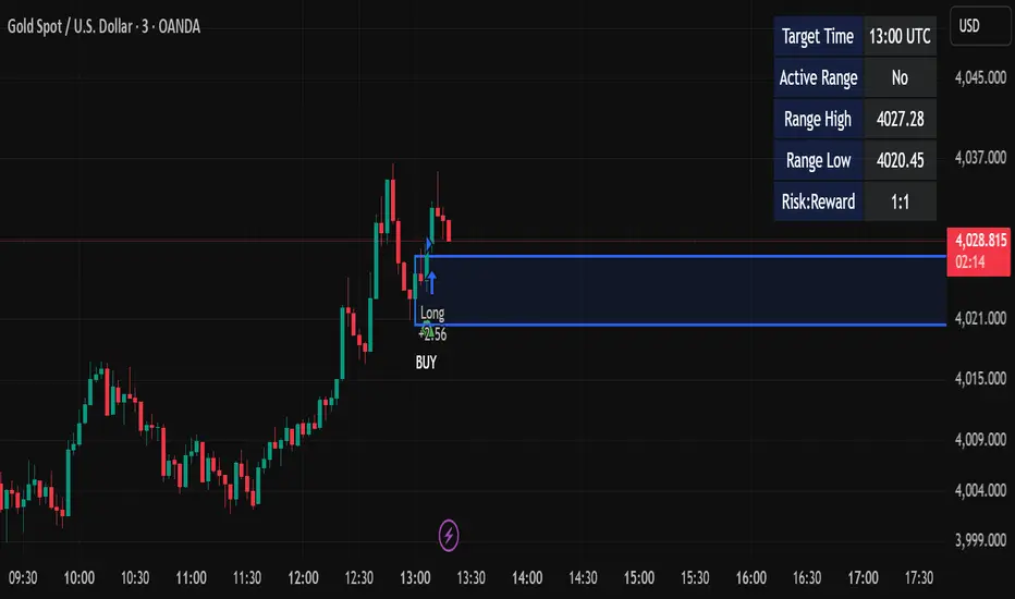
BOCS Channel Scalper Indicator - Mean Reversion Alert System# BOCS Channel Scalper Indicator - Mean Reversion Alert System
## WHAT THIS INDICATOR DOES:
This is a mean reversion trading indicator that identifies consolidation channels through volatility analysis and generates alert signals when price enters entry zones near channel boundaries. **This indicator version is designed for manual trading with comprehensive alert functionality.** Unlike automated strategies, this tool sends notifications (via popup, email, SMS, or webhook) when trading opportunities occur, allowing you to manually review and execute trades. The system assumes price will revert to the channel mean, identifying scalp opportunities as price reaches extremes and preparing to bounce back toward center.
## INDICATOR VS STRATEGY - KEY DISTINCTION:
**This is an INDICATOR with alerts, not an automated strategy.** It does not execute trades automatically. Instead, it:
- Displays visual signals on your chart when entry conditions are met
- Sends customizable alerts to your device/email when opportunities arise
- Shows TP/SL levels for reference but does not place orders
- Requires you to manually enter and exit positions based on signals
- Works with all TradingView subscription levels (alerts included on all plans)
**For automated trading with backtesting**, use the strategy version. For manual control with notifications, use this indicator version.
## ALERT CAPABILITIES:
This indicator includes four distinct alert conditions that can be configured independently:
**1. New Channel Formation Alert**
- Triggers when a fresh BOCS channel is identified
- Message: "New BOCS channel formed - potential scalp setup ready"
- Use this to prepare for upcoming trading opportunities
**2. Long Scalp Entry Alert**
- Fires when price touches the long entry zone
- Message includes current price, calculated TP, and SL levels
- Notification example: "LONG scalp signal at 24731.75 | TP: 24743.2 | SL: 24716.5"
**3. Short Scalp Entry Alert**
- Fires when price touches the short entry zone
- Message includes current price, calculated TP, and SL levels
- Notification example: "SHORT scalp signal at 24747.50 | TP: 24735.0 | SL: 24762.75"
**4. Any Entry Signal Alert**
- Combined alert for both long and short entries
- Use this if you want a single alert stream for all opportunities
- Message: "BOCS Scalp Entry: at "
**Setting Up Alerts:**
1. Add indicator to chart and configure settings
2. Click the Alert (⏰) button in TradingView toolbar
3. Select "BOCS Channel Scalper" from condition dropdown
4. Choose desired alert type (Long, Short, Any, or Channel Formation)
5. Set "Once Per Bar Close" to avoid false signals during bar formation
6. Configure delivery method (popup, email, webhook for automation platforms)
7. Save alert - it will fire automatically when conditions are met
**Alert Message Placeholders:**
Alerts use TradingView's dynamic placeholder system:
- {{ticker}} = Symbol name (e.g., NQ1!)
- {{close}} = Current price at signal
- {{plot_1}} = Calculated take profit level
- {{plot_2}} = Calculated stop loss level
These placeholders populate automatically, creating detailed notification messages without manual configuration.
## KEY DIFFERENCE FROM ORIGINAL BOCS:
**This indicator is designed for traders seeking higher trade frequency.** The original BOCS indicator trades breakouts OUTSIDE channels, waiting for price to escape consolidation before entering. This scalper version trades mean reversion INSIDE channels, entering when price reaches channel extremes and betting on a bounce back to center. The result is significantly more trading opportunities:
- **Original BOCS**: 1-3 signals per channel (only on breakout)
- **Scalper Indicator**: 5-15+ signals per channel (every touch of entry zones)
- **Trade Style**: Mean reversion vs trend following
- **Hold Time**: Seconds to minutes vs minutes to hours
- **Best Markets**: Ranging/choppy conditions vs trending breakouts
This makes the indicator ideal for active day traders who want continuous alert opportunities within consolidation zones rather than waiting for breakout confirmation. However, increased signal frequency also means higher potential commission costs and requires disciplined trade selection when acting on alerts.
## TECHNICAL METHODOLOGY:
### Price Normalization Process:
The indicator normalizes price data to create consistent volatility measurements across different instruments and price levels. It calculates the highest high and lowest low over a user-defined lookback period (default 100 bars). Current close price is normalized using: (close - lowest_low) / (highest_high - lowest_low), producing values between 0 and 1 for standardized volatility analysis.
### Volatility Detection:
A 14-period standard deviation is applied to the normalized price series to measure price deviation from the mean. Higher standard deviation values indicate volatility expansion; lower values indicate consolidation. The indicator uses ta.highestbars() and ta.lowestbars() to identify when volatility peaks and troughs occur over the detection period (default 14 bars).
### Channel Formation Logic:
When volatility crosses from a high level to a low level (ta.crossover(upper, lower)), a consolidation phase begins. The indicator tracks the highest and lowest prices during this period, which become the channel boundaries. Minimum duration of 10+ bars is required to filter out brief volatility spikes. Channels are rendered as box objects with defined upper and lower boundaries, with colored zones indicating entry areas.
### Entry Signal Generation:
The indicator uses immediate touch-based entry logic. Entry zones are defined as a percentage from channel edges (default 20%):
- **Long Entry Zone**: Bottom 20% of channel (bottomBound + channelRange × 0.2)
- **Short Entry Zone**: Top 20% of channel (topBound - channelRange × 0.2)
Long signals trigger when candle low touches or enters the long entry zone. Short signals trigger when candle high touches or enters the short entry zone. Visual markers (arrows and labels) appear on chart, and configured alerts fire immediately.
### Cooldown Filter:
An optional cooldown period (measured in bars) prevents alert spam by enforcing minimum spacing between consecutive signals. If cooldown is set to 3 bars, no new long alert will fire until 3 bars after the previous long signal. Long and short cooldowns are tracked independently, allowing both directions to signal within the same period.
### ATR Volatility Filter:
The indicator includes a multi-timeframe ATR filter to avoid alerts during low-volatility conditions. Using request.security(), it fetches ATR values from a specified timeframe (e.g., 1-minute ATR while viewing 5-minute charts). The filter compares current ATR to a user-defined minimum threshold:
- If ATR ≥ threshold: Alerts enabled
- If ATR < threshold: No alerts fire
This prevents notifications during dead zones where mean reversion is unreliable due to insufficient price movement. The ATR status is displayed in the info table with visual confirmation (✓ or ✗).
### Take Profit Calculation:
Two TP methods are available:
**Fixed Points Mode**:
- Long TP = Entry + (TP_Ticks × syminfo.mintick)
- Short TP = Entry - (TP_Ticks × syminfo.mintick)
**Channel Percentage Mode**:
- Long TP = Entry + (ChannelRange × TP_Percent)
- Short TP = Entry - (ChannelRange × TP_Percent)
Default 50% targets the channel midline, a natural mean reversion target. These levels are displayed as visual lines with labels and included in alert messages for reference when manually placing orders.
### Stop Loss Placement:
Stop losses are calculated just outside the channel boundary by a user-defined tick offset:
- Long SL = ChannelBottom - (SL_Offset_Ticks × syminfo.mintick)
- Short SL = ChannelTop + (SL_Offset_Ticks × syminfo.mintick)
This logic assumes channel breaks invalidate the mean reversion thesis. SL levels are displayed on chart and included in alert notifications as suggested stop placement.
### Channel Breakout Management:
Channels are removed when price closes more than 10 ticks outside boundaries. This tolerance prevents premature channel deletion from minor breaks or wicks, allowing the mean reversion setup to persist through small boundary violations.
## INPUT PARAMETERS:
### Channel Settings:
- **Nested Channels**: Allow multiple overlapping channels vs single channel
- **Normalization Length**: Lookback for high/low calculation (1-500, default 100)
- **Box Detection Length**: Period for volatility detection (1-100, default 14)
### Scalping Settings:
- **Enable Long Scalps**: Toggle long alert generation on/off
- **Enable Short Scalps**: Toggle short alert generation on/off
- **Entry Zone % from Edge**: Size of entry zone (5-50%, default 20%)
- **SL Offset (Ticks)**: Distance beyond channel for stop (1+, default 5)
- **Cooldown Period (Bars)**: Minimum spacing between alerts (0 = no cooldown)
### ATR Filter:
- **Enable ATR Filter**: Toggle volatility filter on/off
- **ATR Timeframe**: Source timeframe for ATR (1, 5, 15, 60 min, etc.)
- **ATR Length**: Smoothing period (1-100, default 14)
- **Min ATR Value**: Threshold for alert enablement (0.1+, default 10.0)
### Take Profit Settings:
- **TP Method**: Choose Fixed Points or % of Channel
- **TP Fixed (Ticks)**: Static distance in ticks (1+, default 30)
- **TP % of Channel**: Dynamic target as channel percentage (10-100%, default 50%)
### Appearance:
- **Show Entry Zones**: Toggle zone labels on channels
- **Show Info Table**: Display real-time indicator status
- **Table Position**: Corner placement (Top Left/Right, Bottom Left/Right)
- **Long Color**: Customize long signal color (default: darker green for readability)
- **Short Color**: Customize short signal color (default: red)
- **TP/SL Colors**: Customize take profit and stop loss line colors
- **Line Length**: Visual length of TP/SL reference lines (5-200 bars)
## VISUAL INDICATORS:
- **Channel boxes** with semi-transparent fill showing consolidation zones
- **Colored entry zones** labeled "LONG ZONE ▲" and "SHORT ZONE ▼"
- **Entry signal arrows** below/above bars marking long/short alerts
- **TP/SL reference lines** with emoji labels (⊕ Entry, 🎯 TP, 🛑 SL)
- **Info table** showing channel status, last signal, entry/TP/SL prices, risk/reward ratio, and ATR filter status
- **Visual confirmation** when alerts fire via on-chart markers synchronized with notifications
## HOW TO USE:
### For 1-3 Minute Scalping with Alerts (NQ/ES):
- ATR Timeframe: "1" (1-minute)
- ATR Min Value: 10.0 (for NQ), adjust per instrument
- Entry Zone %: 20-25%
- TP Method: Fixed Points, 20-40 ticks
- SL Offset: 5-10 ticks
- Cooldown: 2-3 bars to reduce alert spam
- **Alert Setup**: Configure "Any Entry Signal" for combined long/short notifications
- **Execution**: When alert fires, verify chart visuals, then manually place limit order at entry zone with provided TP/SL levels
### For 5-15 Minute Day Trading with Alerts:
- ATR Timeframe: "5" or match chart
- ATR Min Value: Adjust to instrument (test 8-15 for NQ)
- Entry Zone %: 20-30%
- TP Method: % of Channel, 40-60%
- SL Offset: 5-10 ticks
- Cooldown: 3-5 bars
- **Alert Setup**: Configure separate "Long Scalp Entry" and "Short Scalp Entry" alerts if you trade directionally based on bias
- **Execution**: Review channel structure on alert, confirm ATR filter shows ✓, then enter manually
### For 30-60 Minute Swing Scalping with Alerts:
- ATR Timeframe: "15" or "30"
- ATR Min Value: Lower threshold for broader market
- Entry Zone %: 25-35%
- TP Method: % of Channel, 50-70%
- SL Offset: 10-15 ticks
- Cooldown: 5+ bars or disable
- **Alert Setup**: Use "New Channel Formation" to prepare for setups, then "Any Entry Signal" for execution alerts
- **Execution**: Larger timeframes allow more analysis time between alert and entry
### Webhook Integration for Semi-Automation:
- Configure alert webhook URL to connect with platforms like TradersPost, TradingView Paper Trading, or custom automation
- Alert message includes all necessary order parameters (direction, entry, TP, SL)
- Webhook receives structured data when signal fires
- External platform can auto-execute based on alert payload
- Still maintains manual oversight vs full strategy automation
## USAGE CONSIDERATIONS:
- **Manual Discipline Required**: Alerts provide opportunities but execution requires judgment. Not all alerts should be taken - consider market context, trend, and channel quality
- **Alert Timing**: Alerts fire on bar close by default. Ensure "Once Per Bar Close" is selected to avoid false signals during bar formation
- **Notification Delivery**: Mobile/email alerts may have 1-3 second delay. For immediate execution, use desktop popups or webhook automation
- **Cooldown Necessity**: Without cooldown, rapidly touching price action can generate excessive alerts. Start with 3-bar cooldown and adjust based on alert volume
- **ATR Filter Impact**: Enabling ATR filter dramatically reduces alert count but improves quality. Track filter status in info table to understand when you're receiving fewer alerts
- **Commission Awareness**: High alert frequency means high potential trade count. Calculate if your commission structure supports frequent scalping before acting on all alerts
## COMPATIBLE MARKETS:
Works on any instrument with price data including stock indices (NQ, ES, YM, RTY), individual stocks, forex pairs (EUR/USD, GBP/USD), cryptocurrency (BTC, ETH), and commodities. Volume-based features are not included in this indicator version. Multi-timeframe ATR requires higher-tier TradingView subscription for request.security() functionality on timeframes below chart timeframe.
## KNOWN LIMITATIONS:
- **Indicator does not execute trades** - alerts are informational only; you must manually place all orders
- **Alert delivery depends on TradingView infrastructure** - delays or failures possible during platform issues
- **No position tracking** - indicator doesn't know if you're in a trade; you must manage open positions independently
- **TP/SL levels are reference only** - you must manually set these on your broker platform; they are not live orders
- **Immediate touch entry can generate many alerts** in choppy zones without adequate cooldown
- **Channel deletion at 10-tick breaks** may be too aggressive or lenient depending on instrument tick size
- **ATR filter from lower timeframes** requires TradingView Premium/Pro+ for request.security()
- **Mean reversion logic fails** in strong breakout scenarios - alerts will fire but trades may hit stops
- **No partial closing capability** - full position management is manual; you determine scaling out
- **Alerts do not account for gaps** or overnight price changes; morning alerts may be stale
## RISK DISCLOSURE:
Trading involves substantial risk of loss. This indicator provides signals for educational and informational purposes only and does not constitute financial advice. Past performance does not guarantee future results. Mean reversion strategies can experience extended drawdowns during trending markets. Alerts are not guaranteed to be profitable and should be combined with your own analysis. Stop losses may not fill at intended levels during extreme volatility or gaps. Never trade with capital you cannot afford to lose. Consider consulting a licensed financial advisor before making trading decisions. Always verify alerts against current market conditions before executing trades manually.
## ACKNOWLEDGMENT & CREDITS:
This indicator is built upon the channel detection methodology created by **AlgoAlpha** in the "Smart Money Breakout Channels" indicator. Full credit and appreciation to AlgoAlpha for pioneering the normalized volatility approach to identifying consolidation patterns. The core channel formation logic using normalized price standard deviation is AlgoAlpha's original contribution to the TradingView community.
Enhancements to the original concept include: mean reversion entry logic (vs breakout), immediate touch-based alert generation, comprehensive alert condition system with customizable notifications, multi-timeframe ATR volatility filtering, cooldown period for alert management, dual TP methods (fixed points vs channel percentage), visual TP/SL reference lines, and real-time status monitoring table. This indicator version is specifically designed for manual traders who prefer alert-based decision making over automated execution.
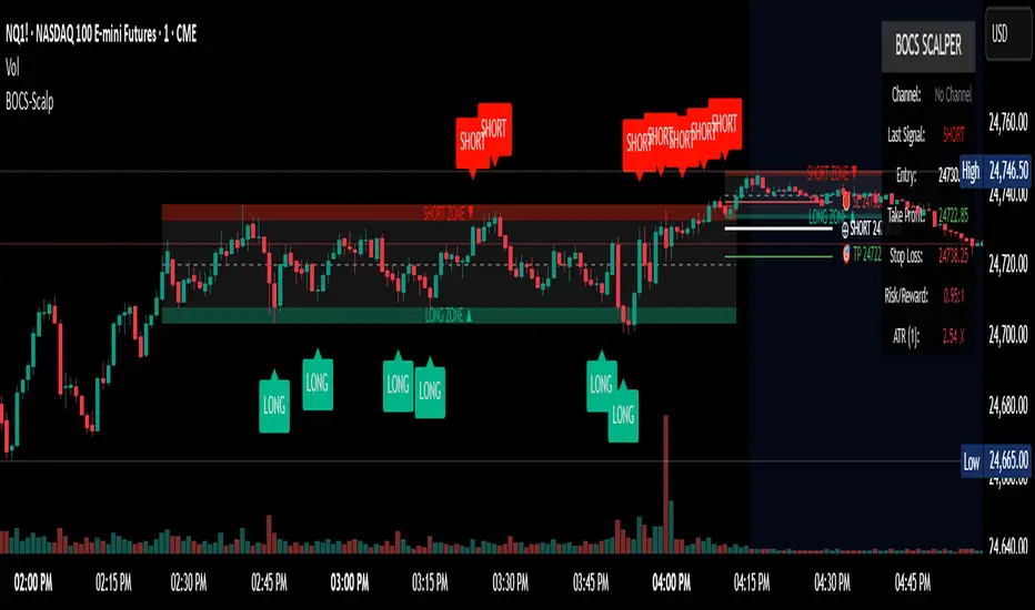
Weekend Hunter Ultimate v6.2 Weekend Hunter Ultimate v6.2 - Automated Crypto Weekend Trading System
OVERVIEW:
Specialized trading strategy designed for cryptocurrency weekend markets (Saturday-Sunday) when institutional traders are typically offline and market dynamics differ significantly from weekdays. Optimized for 15-minute timeframe execution with multi-timeframe confluence analysis.
KEY FEATURES:
- Weekend-Only Trading: Automatically activates during configurable weekend hours
- Dynamic Leverage: 5-20x leverage adjusted based on market safety and signal confidence
- Multi-Timeframe Analysis: Combines 4H trend, 1H momentum, and 15M execution
- 10 Pre-configured Crypto Pairs: BTC, ETH, LINK, XRP, DOGE, SOL, AVAX, PEPE, TON, POL
- Position & Risk Management: Max 4 concurrent positions, -30% account protection
- Smart Trailing Stops: Protects profits when approaching targets
RISK MANAGEMENT:
- Maximum daily loss: 5% (configurable)
- Maximum weekend loss: 15% (configurable)
- Per-position risk: Capped at 120-156 USDT
- Emergency stops for flash crashes (8% moves)
- Consecutive loss protection (4 losses = pause)
TECHNICAL INDICATORS:
- CVD (Cumulative Volume Delta) divergence detection
- ATR-based dynamic stop loss and take profit
- RSI, MACD, Bollinger Bands confluence
- Volume surge confirmation (1.5x average)
- Weekend liquidity adjustments
INTEGRATION:
- Designed for Bybit Futures (0.075% taker fee)
- WunderTrading webhook compatibility via JSON alerts
- Minimum position size: 120 USDT (Bybit requirement)
- Initial capital: $500 recommended
TARGET METRICS:
- Win rate target: 65%
- Average win: 5.5%
- Average loss: 1.8%
- Risk-reward ratio: ~3:1
IMPORTANT DISCLAIMERS:
- Past performance does not guarantee future results
- Leveraged trading carries substantial risk of loss
- Weekend crypto markets have 13% of normal liquidity
- Not suitable for traders who cannot afford to lose their entire investment
- Requires continuous monitoring and adjustment
USAGE:
1. Apply to 15-minute charts only
2. Configure weekend hours for your timezone
3. Set up webhook alerts for automation
4. Monitor performance table in top-right corner
5. Adjust parameters based on your risk tolerance
This is an experimental strategy for educational purposes. Always test with small amounts first and never invest more than you can afford to lose completely.
